Orthogonal Layout
Overview
The orthogonal layout style is a versatile approach designed for arranging undirected graphs. It excels with medium-sized sparse graphs, creating compact, orderly drawings that avoid node overlaps, minimize crossings, and reduce bends. This layout positions the nodes of a graph so that each connecting edge forms a path of alternating horizontal and vertical segments. It’s particularly beneficial for fields like software engineering, database schema visualization, system management, and knowledge representation, where clarity and compactness are paramount.
Orthogonal layouts are favored in engineering due to their ability to depict complex networks clearly. They can be optimized for various objectives, such as minimizing bends or reducing the drawing area. These layouts are applied in areas including software engineering, database schema design, system management, knowledge representation, VLSI circuit design, and floor planning.
The algorithm behind this layout style also accommodates directed edge drawings, enhancing clarity in applications like software engineering, database schema, and system management. However, it’s important to note that directed edge drawings are not compatible with hierarchically nested graphs, the ‘from sketch’ mode, or non-standard layout styles.
Furthermore, the algorithm is capable of handling hierarchically nested graphs, adding another layer of structure to the layout. This feature, however, is not available when using directed edge drawings, the ‘from sketch’ mode, or non-standard layout styles. By offering these options, the orthogonal layout algorithm provides flexibility while ensuring that the resulting graph drawings are both functional and aesthetically pleasing.
Features
The Orthogonal Layout algorithm is a sophisticated system designed to arrange graphs in a visually pleasing and readable manner. It offers a variety of layout styles to cater to different aesthetic and functional requirements. These styles include:
- NORMAL: This style routes the edges in a completely orthogonal fashion while preserving the original node sizes.
- UNIFORM: It ensures a consistent look by maintaining uniform edge lengths and angles.
- BOX: Nodes are arranged within a box-shaped layout, emphasizing a compact and squared appearance.
- MIXED: A combination of orthogonal and non-orthogonal edge routing is used to balance readability and spatial efficiency.
- FIXED_BOX: Similar to BOX, but with fixed node dimensions to accommodate content without distortion.
- FIXED_MIXED: A hybrid approach that maintains fixed node sizes while allowing for a mix of routing styles.
To apply these styles, one would use the layoutStyle method, which configures the algorithm according to the chosen style.
The OrthogonalLayout algorithm is also capable of integrating edge label data into the layout process. By activating the integratedEdgeLabeling method, the algorithm adjusts the positions of nodes and edges to prevent any overlap with edge labels, ensuring that all labels are clearly visible and do not interfere with the graph’s structure.
For more granular control over the layout of individual edges, OrthogonalLayoutEdgeLayoutDescriptor instances can be utilized. These descriptors allow for the specification of edge-specific information, such as distances between nodes. They are associated with the graph through IDataProviders, which are registered using the key EDGE_LAYOUT_DESCRIPTOR_DP_KEY. In the absence of a specific descriptor for an edge, the algorithm defaults to a pre-set descriptor, which can be customized using the edgeLayoutDescriptor method.
The algorithm strives to optimize various objective functions to enhance the graph’s readability and aesthetics. These objectives include minimizing bends in the edges (optimizePerceivedBends), reducing the number of edge crossings (crossingReduction), shortening edge lengths (edgeLengthReduction), and maximizing the number of faces (faceMaximization). However, enabling these optimizations may significantly increase the algorithm’s running time.
In graphs without group nodes, the OrthogonalLayout algorithm can identify and explicitly arrange certain substructures, such as trees, chains, and cycles. This feature allows these structures to stand out and be easily recognized within the graph. The algorithm provides style properties—treeStyle, chainStyle, and cycleStyle—to define how these substructures should be displayed. Additionally, the algorithm can be configured to consider node types, enabling it to group only nodes of the same user-defined type into a substructure.
However, it’s important to note that for graphs containing group nodes, the algorithm does not support features such as substructure detection, directed edges, and edge grouping. This limitation is due to the complexity introduced by the presence of group nodes, which requires a different approach to graph layout. ### Layout
In the planarization phase, the algorithm begins by creating a planar embedding of the graph. This involves positioning the nodes of the graph in a two-dimensional plane in such a way that no edges cross each other. Since most graphs are not inherently planar, the algorithm may add dummy vertices or perform edge splitting to achieve a planar embedding. The goal here is to approximate the non-planar graph as closely as possible while maintaining planarity.
Once a planar embedding is established, the algorithm proceeds to the orthogonalization phase. During this stage, it determines the shape of the edges by calculating the bends and angles. The objective is to represent each edge with a series of horizontal and vertical segments, forming right angles at their intersections. The algorithm assigns each edge a sequence of direction changes (bends) that adhere to the orthogonal grid. It also ensures that the angles between consecutive edges around a node are consistent with the orthogonal representation, typically aiming for 90-degree angles.
The final phase is compaction, where the algorithm assigns exact coordinates to the nodes and edges. The compaction process is crucial as it impacts the final aesthetics and readability of the graph. The algorithm seeks to minimize the area of the drawing while avoiding overlaps and maintaining the orthogonal representation from the previous phase. It adjusts the lengths of the edge segments and repositions the nodes to create a compact layout. The compaction phase is often subject to various optimization criteria, such as minimizing the total edge length or the number of bends.
Throughout these phases, the orthogonal layout algorithm employs sophisticated mathematical and computational techniques to balance the competing demands of aesthetics, readability, and spatial efficiency. The result is a graph drawing where information is conveyed clearly and effectively, with a structured and orderly appearance that facilitates understanding and analysis.
Business Domains
- In the domain of Software Engineering, orthogonal layouts are utilized for the purpose of visualizing class hierarchies, component diagrams, and various other representations of software architecture (UML diagrams). This aids in the clear depiction of the relationships and structures within software systems.
- Pertaining to Database Schema, orthogonal layouts serve to illustrate entity-relationship diagrams and database designs. They provide a structured and clear visualization of the database components and the relationships between them, which is essential for database design and management.
- Within the realm of System Management, orthogonal layouts are employed for creating network diagrams, planning infrastructure, and illustrating the interconnections between different systems (BPMN diagrams). This is crucial for understanding and managing the complex networks that support business operations.
- In Knowledge Representation, orthogonal layouts are used to display concept maps, knowledge graphs, and semantic networks. These layouts help in representing complex sets of knowledge and information in a way that is easy to understand and navigate.
Technical Details
Data
If you have a graph in JSON format you can use our GraphBuilder to import the data as a graph.
Alternatively, you can explicitly create nodes and edges. We’ll generate, for the sake of example, a random graph (you can see the complete example in the playground below):
const nodeCount = 50
const rootNode = graph.createNode()
const nodes: INode[] = [rootNode]

for (let i = 1; i < nodeCount; i++) {
    nodes.push(graph.createNode())
    graph.createEdge(nodes[Math.floor(Math.random() * (i - 1))], nodes[i])
}
Layout
Like all our layout algorithms, applying the layout is straightforward:
const layout = new OrthogonalLayout();
layout.layoutOrientation = "left-to-right"
await graphComponent.morphLayout(layout, '2s')
Note that: - the CompactOrthogonalLayout is a variant of the OrthogonalLayout that tries to arrange nodes in a more compact way - orthogonal edge editing is unrelated to orthogonal layout but allows you to interactively draw or change edges while preserving an orthogonal edge style.
Playgrounds
const nodeCount = 50
const rootNode = graph.createNode()
const nodes: INode[] = [rootNode]
for (let i = 1; i < nodeCount; i++) {
  nodes.push(graph.createNode())
  graph.createEdge(nodes[Math.floor(Math.random() * (i - 1))], nodes[i])
}
const layout = new OrthogonalLayout();
layout.layoutOrientation = "left-to-right"
await graphComponent.morphLayout(layout, '2s')
▸ the compact orthogonal layout on a very large diagram
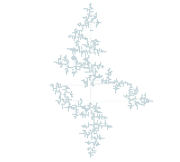
Below you can also see the difference between the compact and standard version.
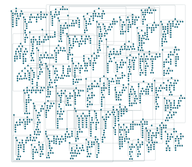
const nodeCount = 1500
const rootNode = graph.createNode()
const nodes: INode[] = [rootNode]
for (let i = 1; i < nodeCount; i++) {
  nodes.push(graph.createNode())
  graph.createEdge(nodes[Math.floor(Math.random() * (i - 1))], nodes[i])
}
const layout = new CompactOrthogonalLayout();
layout.aspectRatio=1.2

await graphComponent.morphLayout(layout, '2s')