States and operators

Quantum states and operators.

• I. Introduction
• II. Elements of quantum mechanics
• III. The electromagnetic field
• IV. The qubit
• V. Quantum gates
• VI. States and operators
• VII. Shor’s algorithm
• VIII. Quantum teleportation
• IX. The Deutsch algorithm
• X. The no-cloning theorem
• XI. About anyons
• XII. About SU(2)
• XIII. Teleportation topology
• XIV. The Simon algorithm
• XV. Superdense coding
• XVI. Chern-Simons theory
• XVII. The toric code
• REF. Some pointers

Having seen some of the typical maths you need in part I and part II we’ll turn now to some Python showing how to simulate quantum systems.

I’ll use below the QuTip Python library but there are other very nice libs out there. Also, if Python is not your cup of tea you can also take a look at this list of QC simulators here, the Liquid F# lib in particular.

States

Creating qubits, bras and kets goes typically likes this:

from qutip import *
import numpy as np
sqrt = np.sqrt
import matplotlib.pyplot as plt
plot = plt.plot
%matplotlib inline
basis(4,0)

which returns the \(|0\rangle\) state in a 4-dimensional space:

\(\begin{pmatrix}1.0 \\ 0.0\\0.0\\0.0 \end{pmatrix}\)

The tangled EPR state is hence

epr = (basis(4,0) + basis(4,3))/sqrt(2)
epr

\(\begin{pmatrix}0.707 \\ 0.0\\0.0\\0.707 \end{pmatrix}\)

We saw earlier that qubits can be represented on a Bloch sphere and the library gives you easy access to visualizations:

bloch = Bloch()
state = sigmaz()*sigmax()*basis(2,0)
bloch.add_states(state)
bloch.show()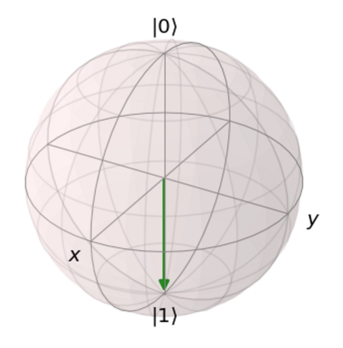

The sigmax, sigmay, sigmaz above are the Pauli spin matrices. Turning the states into a density matrix can be done with the ket2dm command:

ket2dm(epr)

\(\begin{pmatrix}0.5 & 0.0 & 0.0 & 0.5\\ 0.0 & 0.0 & 0.0 & 0.0\\0.0 & 0.0 & 0.0 & 0.0\\0.5 & 0.0 & 0.0 & 0.5 \end{pmatrix}\)

Remember that this is nothing but turning an arbitrary ket \(|\psi\rangle\) into a matrix \(|\psi\rangle\langle\psi|\).

Tensor products are obtained using the tensor method. For example, creating the tensor product of \(\sigma_x\otimes\sigma_y\):

tensor(sigmax(),sigmay())

\(\begin{pmatrix}0.0 & 0.0 & 0.0 & -1.0j\\ 0.0 & 0.0 & 1.0j & 0.0\\0.0 & -1.0j & 0.0 & 0.0\\1.0j & 0.0 & 0.0 & 0.0 \end{pmatrix}\)

so, \((\sigma_x\otimes\sigma_y)(|1\rangle\otimes|0\rangle)\) is hence

t = tensor(sigmax(),sigmay())
t*tensor(basis(2,1), basis(2,0))

\(\begin{pmatrix}0.0 \\ 1.0j\\0.0\\0.0 \end{pmatrix}\).

Operators

Operators are created via the Qobj

op = Qobj([[0,5j], [-5j,0]])

and applied via multiplication on a state

op*(basis(2,0) + basis(2,1))

\(\begin{pmatrix}5.0j \\ -5.0j \end{pmatrix}\).

Eigenstates and eigenvalues are fetched via the eigenstates method on the operator

eig = sy.eigenstates()
print("The eingenvalues %s has eigenvector"%eig[0][0])
eig[1][0]

\(\begin{pmatrix}-0.707j \\ -0.707j \end{pmatrix}\).

Fock space mechanics works as should be and you can check e.g. that \(a^\dagger|0\rangle = |1\rangle\)

create(2)*basis(2,0) == basis(2,1)
True

Similarly, \(a^\dagger a^\dagger|0\rangle = 0\) since \(\{a^\dagger, a^\dagger\}=0\):

create(2)*create(2)*basis(2,0) 

\(\begin{pmatrix}0.0 \\ 0.0 \end{pmatrix}\).

Dynamics

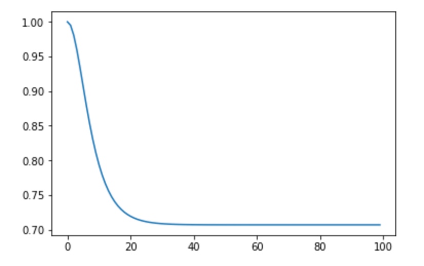
The framework allows you to simulate the evolution of kets or observables using the Lindblad or master equation. For example, the following simple Hamiltonian

\(\hat{H} = \sigma_x\sigma_z\)

evolution on the \(|0\rangle\) ket gives:

H = sigmax()*sigmaz()
psi0 = basis(2, 0)
# list of times for which the solver should store the state vector
tlist = np.linspace(0, 10, 100)
result = mesolve(H, psi0, tlist, [], [])
plot([np.absolute(x[0][0]) for x in result.states])