B = rep(0, 10)
B2 = rep(0, 10)
dt = .1
for(k in 1:100){
 delta = rnorm(10, 0, sqrt(dt))
 B = B + delta
 B2 = B2 + delta^2
}

mean(B2)
[1] 9.643994The rules for random things are somewhat different than the ones you know for ‘smooth’ things. In a university course you get proofs based on Martingales, Wiener measures and whatnot but it all can feel very abstract. Even the basic examples can be confusing. So, here I want to show you that without knowing any high-tech maths you can see from basic examples in R how and that it works.
At the core of it all are random numbers and due to some deep theorems you can safely go with random normal distributions of random numbers, i.e. use the rnorm command. A random walk is simply what it says; a random increment at each step of a series.
If you perform some experiments with the following code:
B = rep(0, 10)
B2 = rep(0, 10)
dt = .1
for(k in 1:100){
delta = rnorm(10, 0, sqrt(dt))
B = B + delta
B2 = B2 + delta^2
}
mean(B2) [1] 9.643994you will quickly recognize that the mean is always close to the total time between start and finish (or the amount of steps T in the loop if you prefer). Using \(\mathbb{E}\) for the mean you get
\(\mathbb{E}(B^2) = T\)
The average distance travelled by a random walk is proportional to the time walking around. The letter B is often used since a random walk is usually called a Brownian process. Also known as a Wiener process.
A very similar result which underlines the crucial difference between smooth number series and random numbers is the following:
dt = .1
B = cumsum(rnorm(1000, 0, sqrt(dt)))
plot(B, t="l")
Bup = cumsum(B*c(0, diff(B,1)))
Bdown = cumsum(B*c(diff(B,1),0))
plot(Bup, col="red", t="l")
par(new=T)
plot(Bdown, col="green", t="l")
par(new=T)
plot(Bup- Bdown, col="grey", t="l")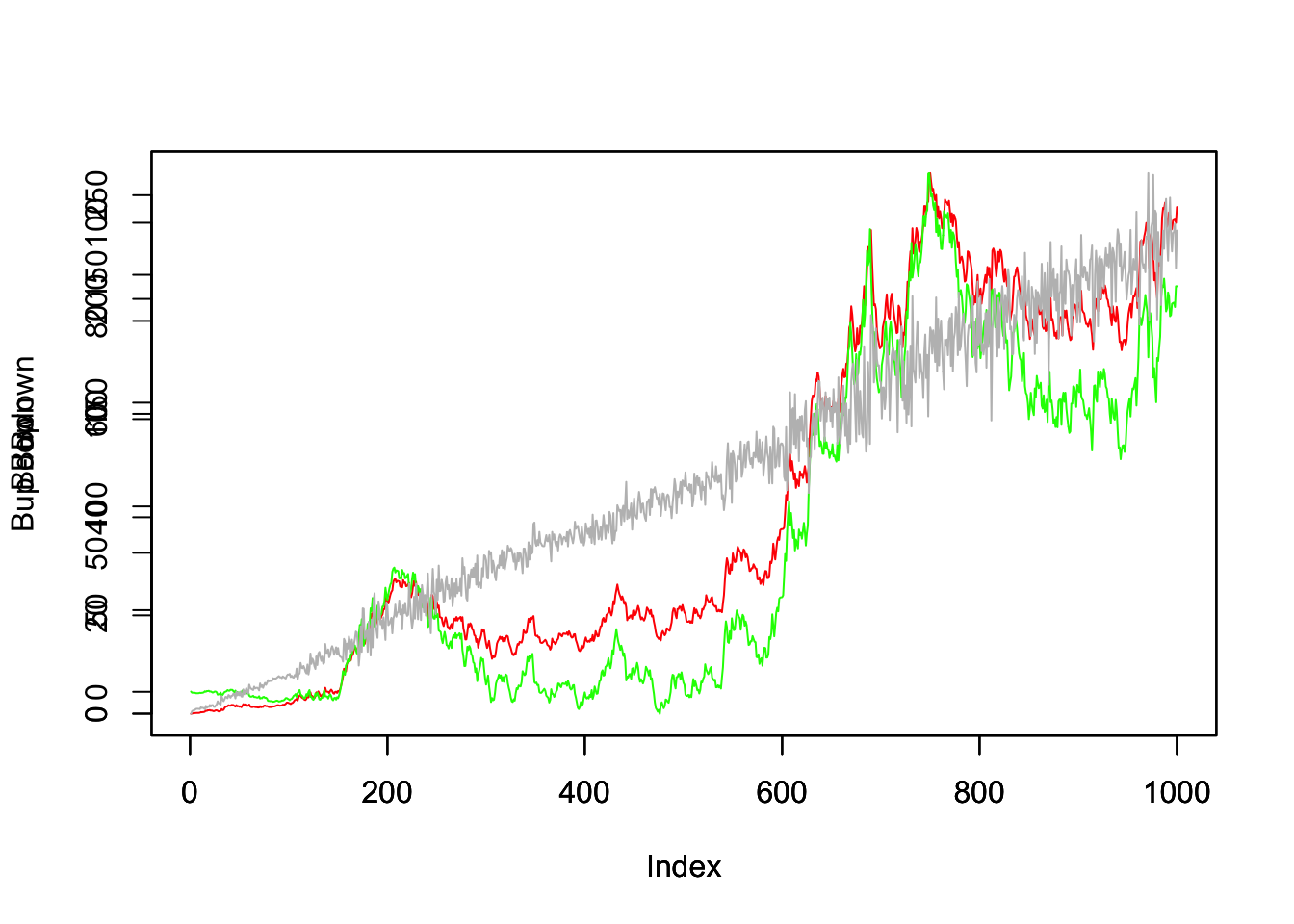
This is a visual proof if you wish that \(\sum_k B_{k+1}(B_{k+1} - B_k)\) and \(\sum_k B_{k}(B_{k+1} - B_k)\) are not the same sums and that contrary to the smooth case they also don’t get closer as the time step decreases. In fact, the guy line indicates that the difference of the two series is proportional to the time
\(\mathbb{E}(\sum_k (B_{k+1} - B_k)^2) = e - s\)
where e, s are the end and start times respectively. This has big consequences. If you would deal with smooth function you would solve the integral (being just a sum of small quantities) like
\(\int b \,db = \frac{b^2}{2}\)
while in the case of random numbers you have an extra term proportional to the time
\(\int B \,dB = \frac{b^2}{2} - \frac{t}{2}\).
Complementary to this, if you wish to have derivatives and differentials of random variables you need an extra term:
\(d(f(B).g(B)) = df(B).g + f(B).dg(B) + df(B).dg(B)\)
where the last term is proportional to the time since \(B^2 \sim T\). How does it work on a concrete example? Let’s say you have the most basic stock price evolution S(t) based on the following stochastic differential equation
\(dS(t) = a\,S(t)\,dt + \sigma\,S(t)\,dB_t\)
and take \(a = 0.3, \sigma = 0.4\) with a starting price of 100:
dt = .1
B = cumsum(rnorm(1000, 0, sqrt(dt)))
S = rep(0,1000)
S[1] = 100
for(t in 2:1000){
 S[t] = S[t-1]*(1+ 0.3*dt + 0.4*(B[t] - B[t-1]))
}
plot(S, col="orange", t="l")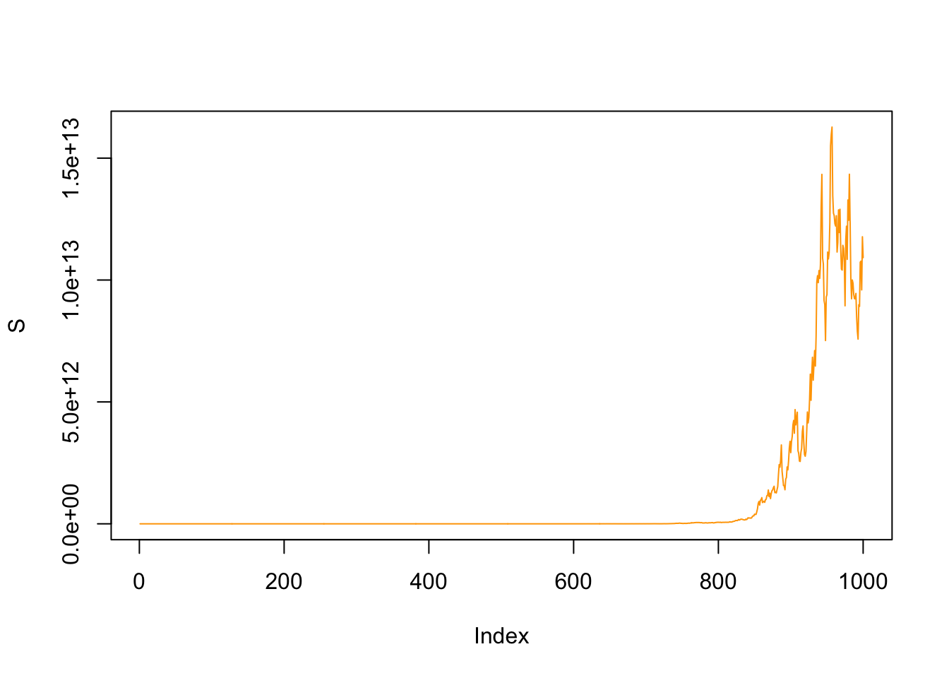
There clearly is an exponential evolution in this plot, so let’s perform a logarithmic transformation \(z=ln(S)\). Since
\((dS)^2 = \sigma^2\,S^2\,dt\)
we get
\(dz = \frac{dS}{S} - \frac{\sigma^2}{2}\,dt\)
and if you work this out a bit more based on the definition of the stock process you get
\(z(t) = (a - - \frac{\sigma^2}{2})\, t + \sigma\, (B_t- B_0) + z(0)\)
and
\(S(t) = C\, exp((a - \frac{\sigma^2}{2})\, t + \sigma\, B_t)\)
which is quite remarkable. It literally says that the loop in our little R program can be replaced with any time interval and without incrementing the series. The constant C can be computed from the initial stock price as
\(S(0) = 100 = C\, exp(0.4\,B_1)\)
So, we rewrite the stock evolution as follows and overlap the two plots
C = 100*exp(-0.4*B[1])
Sol = rep(0, 1000)
for(t in 1:1000){
 Sol[t] = C*exp(0.22*dt*t+0.4*B[t])
}

plot(S[1:200], col="green", t="l")
par(new=T)
plot(Sol[1:200], col="red", t="l")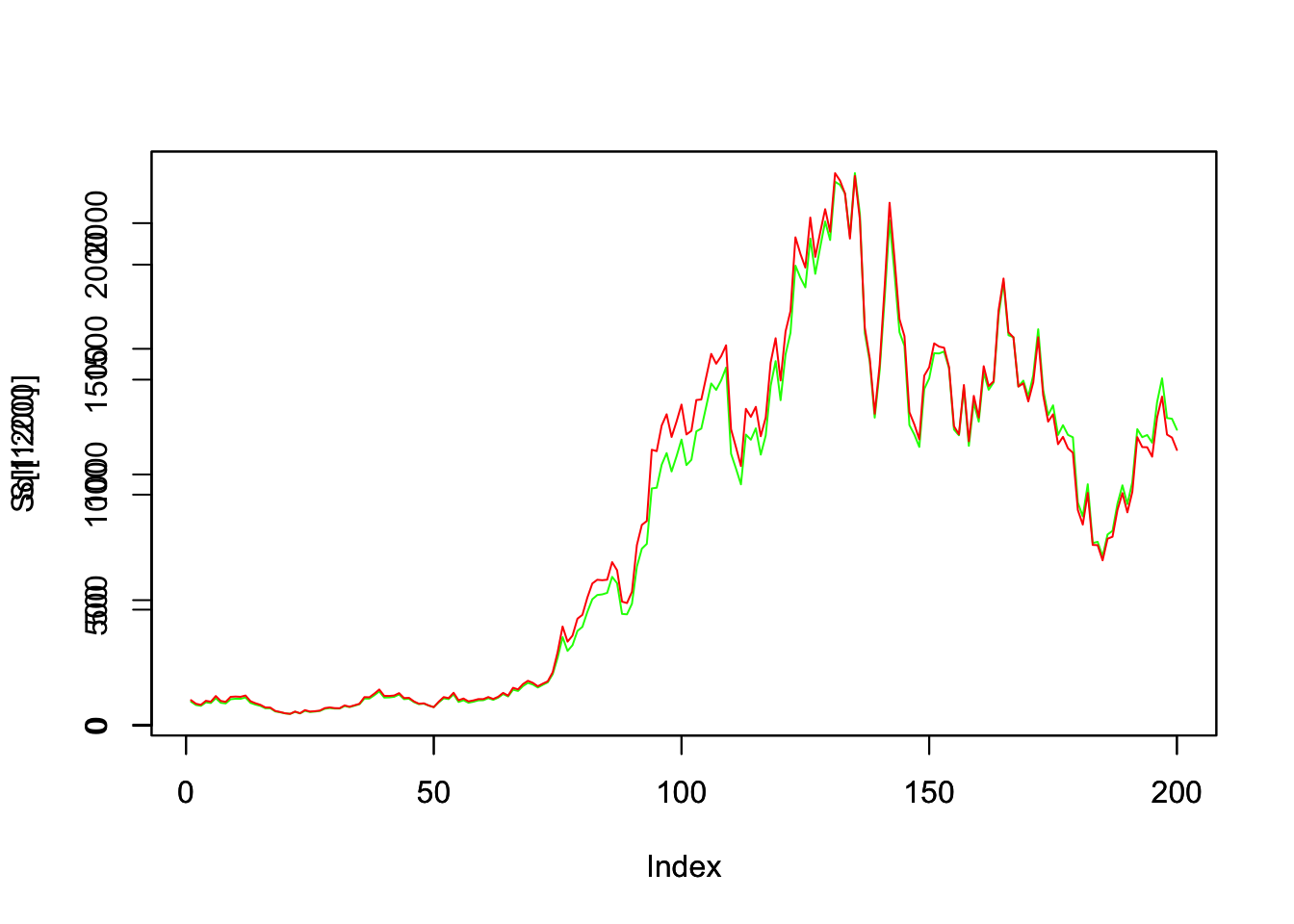
This visually proves the calculation rules described above. If you would ignore the additional term in the integration (or differentiation) as one would in the smooth case you obviously would not have the two plots overlapping.