Jaccard similarity using GDS

In a related note on entity resolution we highlighted how Jaccard similarity can be used as a simple link prediction or similarity measure. In this note we show how within Neo4j you can quickly compute Jaccard via GDS.

You can use the GDS procedures inside the Neo4j browser but here we’ll go via the Python client.

Note that this client is a wrapper around the GDS procedures, you need to have it installed on the database prior to using the client.

URL = "bolt://localhost:7687"
auth = ("neo4j", "123456789")

If all is well, the following should print out the GDS version:

from graphdatascience import GraphDataScience
gds = GraphDataScience(URL, auth=auth)

print(gds.version())

2.9.0

The following is some dummy data:

gds.run_cypher("""
CREATE
  (alice:Person {name: 'Alice'}),
  (bob:Person {name: 'Bob'}),
  (carol:Person {name: 'Carol'}),
  (dave:Person {name: 'Dave'}),
  (eve:Person {name: 'Eve'}),
  (guitar:Instrument {name: 'Guitar'}),
  (synth:Instrument {name: 'Synthesizer'}),
  (bongos:Instrument {name: 'Bongos'}),
  (trumpet:Instrument {name: 'Trumpet'}),

  (alice)-[:LIKES]->(guitar),
  (alice)-[:LIKES]->(synth),
  (alice)-[:LIKES {strength: 0.5}]->(bongos),
  (bob)-[:LIKES]->(guitar),
  (bob)-[:LIKES]->(synth),
  (carol)-[:LIKES]->(bongos),
  (dave)-[:LIKES]->(guitar),
  (dave)-[:LIKES {strength: 1.5}]->(trumpet),
  (dave)-[:LIKES]->(bongos);
               """)

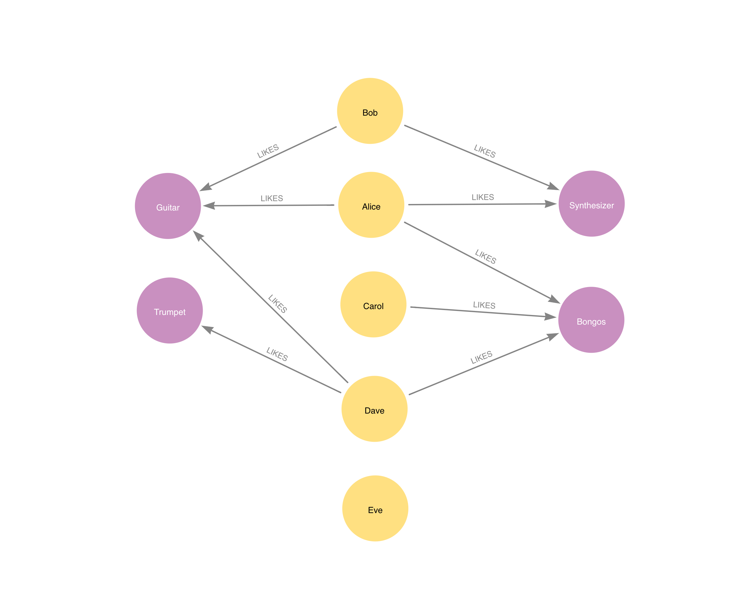
which looks like the following

This simple data is representative for what Jaccard tries to achieve: the more two nodes have neighbors in common, the more they are similar.

To proceed with GDS one has to project the data into a virtual/memory graph:

G, result = gds.graph.cypher.project(
    """
    MATCH (source:Person)
    OPTIONAL MATCH (source)-[r:LIKES]->(target:Instrument)
    RETURN gds.graph.project(
    'myGraph',
    source,
    target,
    { relationshipProperties: r { strength: coalesce(r.strength, 1.0) } }
)
    """,                   #  Cypher query
    database="neo4j",      #  Target database
    graph_name="myGraph",  #  Query parameter
  
)

assert G.node_count() == result["nodeCount"]

GDS has four execution channels and mutate alters the projected data without changing the database:

gds.nodeSimilarity.mutate(G, mutateRelationshipType="SIMILAR", mutateProperty="score", similarityCutoff=0)

preProcessingMillis                                                       0
computeMillis                                                             3
mutateMillis                                                              5
postProcessingMillis                                                      0
nodesCompared                                                             4
relationshipsWritten                                                     12
similarityDistribution    {'min': 0.0, 'p5': 0.0, 'max': 0.6666679382324...
configuration             {'mutateProperty': 'score', 'jobId': '9793e7e1...
Name: 0, dtype: object

Note that you don’t need to mutate before the write (see below). This method is useful if you wish to accumulate changes in memory, say, as part of a pipeline. There is no direct way to use Cypher on projected graphs (it used to be but got deprecated), you can use however things like the gds.graph.nodeProperty.stream utility to inspect changes.

The stream method returns the algorithm without changing the projected graph or the underlying one:

gds.nodeSimilarity.stream(G,  topK=1 )

	node1	node2	similarity
0	0	1	0.571429
1	1	0	0.571429
2	2	0	0.428571
3	3	0	0.500000

Finally, you can write the similarity to the real graph like so:

gds.nodeSimilarity.write(G, writeRelationshipType= 'SIMILAR',  writeProperty= 'score',  topK=1 )

preProcessingMillis                                                       0
computeMillis                                                             1
writeMillis                                                              12
postProcessingMillis                                                      0
nodesCompared                                                             4
relationshipsWritten                                                      4
similarityDistribution    {'min': 0.4285697937011719, 'p5': 0.4285697937...
configuration             {'writeProperty': 'score', 'writeRelationshipT...
Name: 0, dtype: object

The results are not surprising, just by looking at the image above one could compute the Jaccard coefficient. The topK parameter picks up the most similar sibling for each node.

If you want to use a threshold or refine the similarity, the nodeSimilarity has a sub-method where you can supply things like a minimum degree or a similariy threshold:

gds.nodeSimilarity.filtered.stream(G,similarityCutoff=0.5 )

	node1	node2	similarity
0	0	1	0.571429
1	0	3	0.500000
2	1	0	0.571429
3	3	0	0.500000