NetworkX Overview

Graphs

A tutorial on NetworkX

NetworkX is a comprehensive Python library designed for the creation, manipulation, and study of complex networks and graphs. It provides tools to work with both simple and complex graph structures, including directed and undirected graphs, multigraphs, and more. NetworkX supports a wide range of graph algorithms, such as shortest path, clustering, and network flow, making it suitable for various applications in social network analysis, biology, computer science, and more. The library is highly flexible and integrates well with other scientific computing libraries like NumPy and SciPy, allowing for efficient computation and analysis of large-scale networks.

Setup

# !pip install faker
import networkx as nx
import matplotlib.pyplot as plt
from faker import Faker
faker = Faker()
%matplotlib inline

Creating graphs

Make sure that you understand what the scope is of a particular graph instance. The graph algorithms in NetworkX usually apply only to a few types of graphs. There are, however, method which convert things. E.g. to convert a directed graph to an undirected you would use something like this

G_directed = nx.DiGraph()
G_directed.add_edges_from([(1, 2), (2, 3), (3, 1)])
G_undirected = G_directed.to_undirected()

Instantiating a graph is as simple as:

# default
G = nx.Graph()
# an empty graph
EG = nx.empty_graph(100)
# a directed graph
DG = nx.DiGraph()
# a multi-directed graph
MDG = nx.MultiDiGraph()
# a complete graph
CG = nx.complete_graph(10)
# a path graph
PG = nx.path_graph(5)
# a complete bipartite graph
CBG = nx.complete_bipartite_graph(5,3)
# a grid graph
GG = nx.grid_graph([2, 3, 5, 2])

Analysis

Creating and visualizing a basic graph requires more than one would expect:

import random

gr = nx.DiGraph()
gr.add_node(1, data={'label': 'Space'})
gr.add_node(2, data={'label': 'Time'})
gr.add_node(3, data={'label': 'Gravitation'})
gr.add_node(4, data={'label': 'Geometry'})
gr.add_node(5, data={'label': 'SU(2)'})
gr.add_node(6, data={'label': 'Spin'})
gr.add_node(7, data={'label': 'GL(n)'})
edge_array = [(1, 2), (2, 3), (3, 1), (3, 4), (2, 5), (5, 6), (1, 7)]
gr.add_edges_from(edge_array)
for e in edge_array:
    nx.set_edge_attributes(gr, {e: {'data':{'weight': round(random.random(),2)}}})
    gr.add_edge(*e, weight=round(random.random(),2))
    labelDic = {n:gr.nodes[n]["data"]["label"] for n in gr.nodes()}
    edgeDic = {e:gr.edges[e]["weight"] for e in G.edges}
kpos = nx.layout.kamada_kawai_layout(gr)
nx.draw_networkx(gr,kpos,  labels = labelDic, with_labels=True, arrowsize=25)
o=nx.draw_networkx_edge_labels(gr, kpos, edge_labels= edgeDic, label_pos=0.4)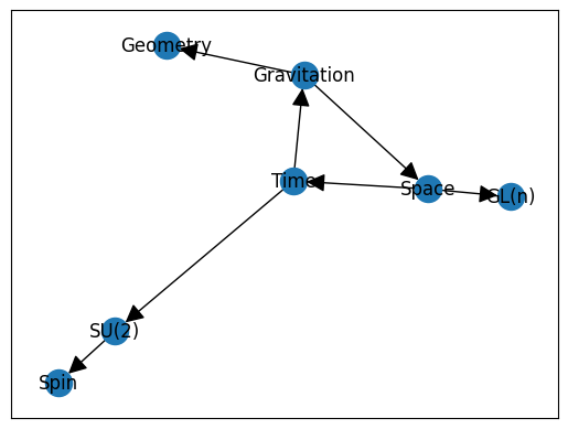

If you want to turn to Numpy

nx.adjacency_matrix(gr).todense()

matrix([[0.  , 0.18, 0.  , 0.  , 0.  , 0.  , 0.13],
        [0.  , 0.  , 0.44, 0.  , 0.75, 0.  , 0.  ],
        [0.61, 0.  , 0.  , 0.27, 0.  , 0.  , 0.  ],
        [0.  , 0.  , 0.  , 0.  , 0.  , 0.  , 0.  ],
        [0.  , 0.  , 0.  , 0.  , 0.  , 0.28, 0.  ],
        [0.  , 0.  , 0.  , 0.  , 0.  , 0.  , 0.  ],
        [0.  , 0.  , 0.  , 0.  , 0.  , 0.  , 0.  ]])

The spectrum of the graph:

nx.adjacency_spectrum(gr)

array([-0.18210492+0.31541497j, -0.18210492-0.31541497j,
        0.36420984+0.j        ,  0.        +0.j        ,
        0.        +0.j        ,  0.        +0.j        ,
        0.        +0.j        ])

and the Laplacian of this graph:

nx.laplacian_matrix(gr.to_undirected()).todense()

matrix([[ 1.52, -0.41, -0.47,  0.  ,  0.  ,  0.  , -0.64],
        [-0.41,  1.22, -0.28,  0.  , -0.53,  0.  ,  0.  ],
        [-0.47, -0.28,  1.4 , -0.65,  0.  ,  0.  ,  0.  ],
        [ 0.  ,  0.  , -0.65,  0.65,  0.  ,  0.  ,  0.  ],
        [ 0.  , -0.53,  0.  ,  0.  ,  0.8 , -0.27,  0.  ],
        [ 0.  ,  0.  ,  0.  ,  0.  , -0.27,  0.27,  0.  ],
        [-0.64,  0.  ,  0.  ,  0.  ,  0.  ,  0.  ,  0.64]])

nx.attr_matrix(gr, edge_attr="weight")

(matrix([[0.  , 0.18, 0.  , 0.  , 0.  , 0.  , 0.13],
         [0.  , 0.  , 0.44, 0.  , 0.75, 0.  , 0.  ],
         [0.61, 0.  , 0.  , 0.27, 0.  , 0.  , 0.  ],
         [0.  , 0.  , 0.  , 0.  , 0.  , 0.  , 0.  ],
         [0.  , 0.  , 0.  , 0.  , 0.  , 0.28, 0.  ],
         [0.  , 0.  , 0.  , 0.  , 0.  , 0.  , 0.  ],
         [0.  , 0.  , 0.  , 0.  , 0.  , 0.  , 0.  ]]),
 [1, 2, 3, 4, 5, 6, 7])

It’s common to use a centrality measure for the size of nodes:

cent = nx.centrality.betweenness_centrality(gr)
nx.draw_networkx(gr, node_size=[v * 1500 for v in cent.values()], edge_color='silver')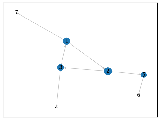

The weakly connected components

nx.is_connected(gr.to_undirected())
comps = nx.components.connected_components(gr.to_undirected())
for c in comps:
    print(c)

{1, 2, 3, 4, 5, 6, 7}

def show_clique(graph, k = 4):
    '''
        Draws the first clique of the specified size.
    '''
    cliques = list(nx.algorithms.find_cliques(graph))
    kclique = [clq for clq in cliques if len(clq) == k]
    if len(kclique)>0:
        print(kclique[0])
        cols = ["red" if i in kclique[0] else "white" for i in graph.nodes() ]
        nx.draw_networkx(graph, with_labels=True, node_color= cols, edge_color="silver")
        return nx.subgraph(graph, kclique[0])
    else:
        print("No clique of size %s."%k)
        return nx.Graph()

ba = nx.barabasi_albert_graph(50, 5)
subg = show_clique(ba,5)
nx.is_isomorphic(subg, nx.complete_graph(5))

[1, 7, 8, 5, 9]

True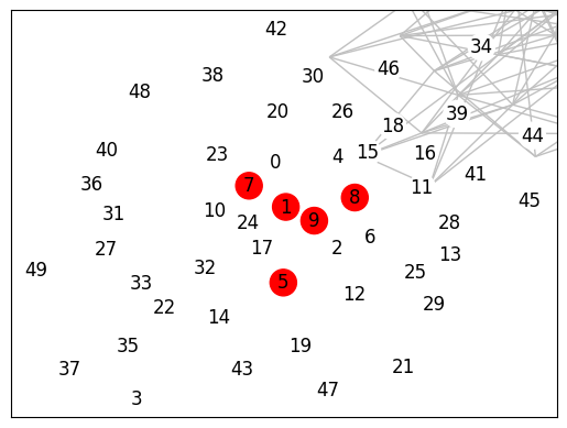

Set data

Often one wishes the nodes and edges to carry a payload:

G = nx.Graph()
G.add_node(12)
nx.set_node_attributes(G, {12:{'payload':{'id': 44, 'name': 'Swa' }}})
print(G.nodes[12]['payload'])
print(G.nodes[12]['payload']['name'])

{'id': 44, 'name': 'Swa'}
Swa

Pandas

The interplay between Pandas and NetworkX is also often crucial in an analysis:

g = nx.barabasi_albert_graph(50, 5)
# set a weight on the edges
for e in g.edges:
    nx.set_edge_attributes(g, {e: {'weight':faker.random.random()}})
for n in g.nodes:
    nx.set_node_attributes(g, {n: {"feature": {"firstName": faker.first_name(), "lastName": faker.last_name()}}})

nx.to_pandas_edgelist(g)

	source	target	weight
0	0	5	0.922816
1	0	6	0.628166
2	0	9	0.947202
3	0	11	0.696823
4	0	20	0.998949
...	...	...	...
220	36	41	0.347691
221	36	47	0.417671
222	38	46	0.675554
223	38	49	0.161978
224	41	46	0.775454

225 rows × 3 columns

import pandas as pd
import copy
node_dic = {id:g.nodes[id]["feature"] for id in g.nodes} # easy acces to the nodes
rows = [] # the array we'll give to Pandas
for e in g.edges:
    row = copy.copy(node_dic[e[0]])
    row["sourceId"] = e[0]
    row["targetId"] = e[1]
    row["weight"] = g.edges[e]["weight"]
    rows.append(row)
df = pd.DataFrame(rows)
df

	firstName	lastName	sourceId	targetId	weight
0	Julie	Aguirre	0	5	0.922816
1	Julie	Aguirre	0	6	0.628166
2	Julie	Aguirre	0	9	0.947202
3	Julie	Aguirre	0	11	0.696823
4	Julie	Aguirre	0	20	0.998949
...	...	...	...	...	...
220	William	Garcia	36	41	0.347691
221	William	Garcia	36	47	0.417671
222	Jane	Gray	38	46	0.675554
223	Jane	Gray	38	49	0.161978
224	Eric	Morgan	41	46	0.775454

225 rows × 5 columns

Visualization

NetworkX is on its own very bad in visualizing graphs. Its strength are the algorithms on and not the display of graphs. If you want to have pretty pictures there are some options:

within Jupyter you can use iPyCytoscape
VisJs also has a Jupyter PyVis widget
for more advanced graph layout you should consider the yFiles graph widget
you can export NetworkX graphs to GML, GraphML and other formats which can be imported in Gephi, yFiles Online and yEd. See our article on Cora for more details.

The last option gives the best results but it means your data is disconnected from the main flow of your Jupyter notebook.