Cora Dataset

The Cora dataset consists of 2708 scientific publications classified into one of seven classes. The citation network consists of 5429 links. Each publication in the dataset is described by a 0/1-valued word vector indicating the absence/presence of the corresponding word from the dictionary. The dictionary consists of 1433 unique words.

This dataset is the MNIST equivalent in graph learning and we explore it somewhat explicitly here in function of other articles using again and again this dataset as a testbed.

• Direct link to download the Cora dataset
• Alternative link to download the Cora dataset
• GraphML file with applied layout (same as image above)
• The nodes in CSV format
• The edges in CSV format
• Neo4j v5.2 dump to restore (works with v5.9 and below)

NetworkX

Download and unzip, say in ~/data/cora/:

import os
import networkx as nx
import pandas as pd
data_dir = os.path.expanduser("~/data/cora")

import the edges:

edgelist = pd.read_csv(os.path.join(data_dir, "cora.cites"), sep='\t', header=None, names=["target", "source"])
edgelist["label"] = "cites"

The edgelist is a simple table with the source citing the target. All edges have the same label:

edgelist.sample(frac=1).head(5)

	target	source	label
3876	94229	1111733	cites
3939	101660	1107095	cites
1280	6213	6155	cites
574	2440	1117786	cites
3827	89308	103528	cites

Create a NetworkX graph from thie edge-list:

Gnx = nx.from_pandas_edgelist(edgelist, edge_attr="label")
nx.set_node_attributes(Gnx, "paper", "label")

A typical node looks like

Gnx.nodes[1103985]

{'label': 'paper'}

The data attached to the nodes consists of flags indicating whether a word in a 1433-long dictionary is present or not:

feature_names = ["w_{}".format(ii) for ii in range(1433)]
column_names =  feature_names + ["subject"]
node_data = pd.read_csv(os.path.join(data_dir, "cora.content"), sep='\t', header=None, names=column_names)

Each node has a subject and 1433 other flags corresponding to word occurence:

node_data.head(5)

	w_0	w_1	w_2	w_3	w_4	w_5	w_6	w_7	w_8	w_9	...	w_1424	w_1425	w_1426	w_1427	w_1428	w_1429	w_1430	w_1431	w_1432	subject
31336	0	0	0	0	0	0	0	0	0	0	...	0	0	1	0	0	0	0	0	0	Neural_Networks
1061127	0	0	0	0	0	0	0	0	0	0	...	0	1	0	0	0	0	0	0	0	Rule_Learning
1106406	0	0	0	0	0	0	0	0	0	0	...	0	0	0	0	0	0	0	0	0	Reinforcement_Learning
13195	0	0	0	0	0	0	0	0	0	0	...	0	0	0	0	0	0	0	0	0	Reinforcement_Learning
37879	0	0	0	0	0	0	0	0	0	0	...	0	0	0	0	0	0	0	0	0	Probabilistic_Methods

5 rows × 1434 columns

The different subjects are:

set(node_data["subject"])

{'Case_Based',
 'Genetic_Algorithms',
 'Neural_Networks',
 'Probabilistic_Methods',
 'Reinforcement_Learning',
 'Rule_Learning',
 'Theory'}

A typical ML challenges with this dataset in mind:

• label prediction: predict the subject of a paper (node) on the basis of the surrounding node data and the structure of the graph
• edge prediction: given node data, can one predict the papers that should be cited?

You will find on this site plenty of articles which are based on the Cora dataset.

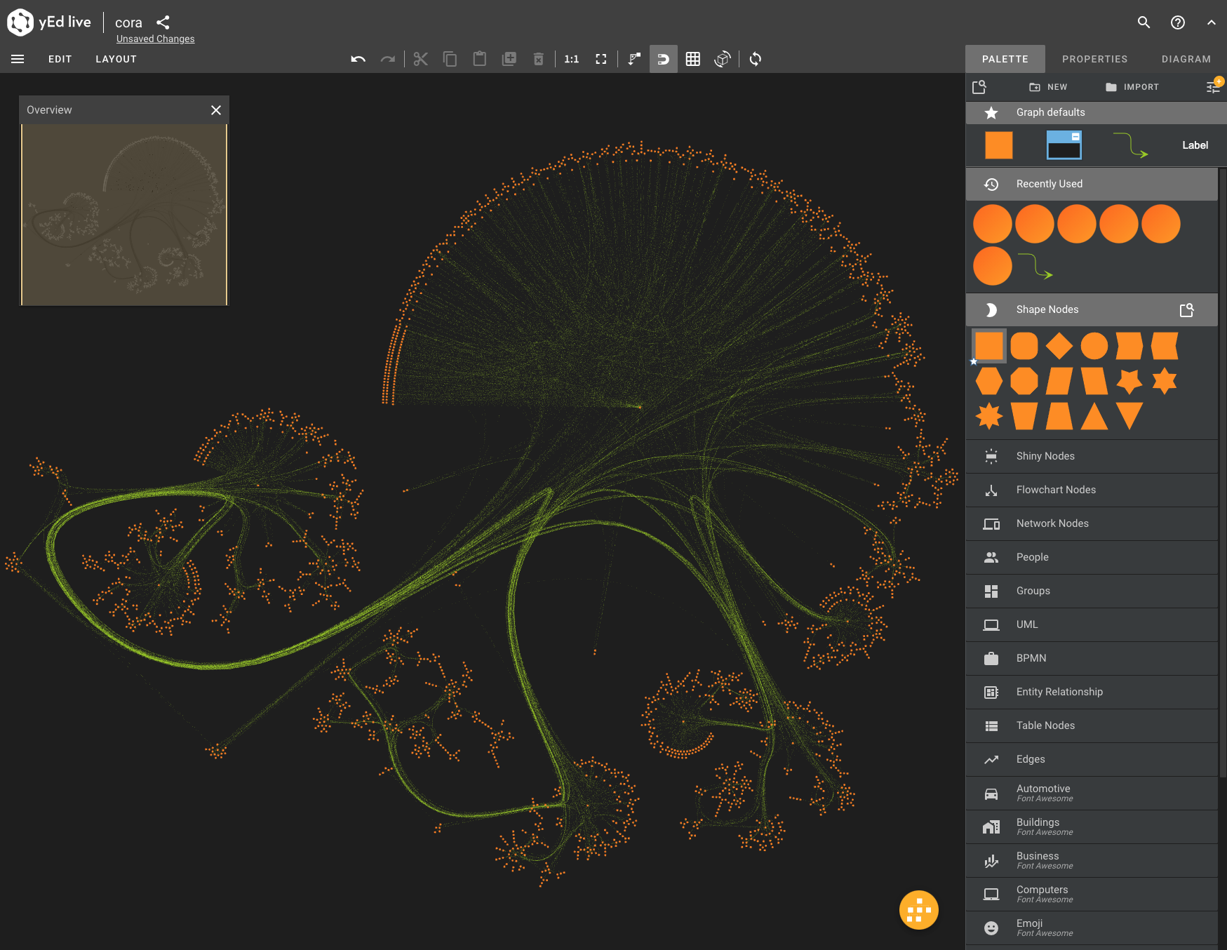
For your information, the visualization above was created via an export of the Cora network to GML (Graph Markup Language), an import into yEd and a balloon layout. It shows some interesting characteristics which can best be analyzed via centrality.

Wolfram

The TSV-formatted datasets linked above are easily loaded into Mathematica and it’s also a lot of fun to apply the black-box machine learning functionality on Cora. As an example, you can find in this gist an edge-prediction model based on node-content and adjacency. The model is poor (accuracy around 70%) but has potential, especially considering how easy it is to experiment within Mathematica.

The Wofram Cora experiment notebook

Pytorch

PyTorch Geometric has various graph datasets and it’s straightforward to download Cora:

from torch_geometric.datasets import Planetoid
dataset = Planetoid(root='~/somewhere/Cora', name='Cora')

data = dataset[0]
print(f'Dataset: {dataset}:')
print('======================')
print(f'Number of graphs: {len(dataset)}')
print(f'Number of features: {dataset.num_features}')
print(f'Number of classes: {dataset.num_classes}')

print(f'Number of nodes: {data.num_nodes}')
print(f'Number of edges: {data.num_edges}')
print(f'Average node degree: {data.num_edges / data.num_nodes:.2f}')
print(f'Number of training nodes: {data.train_mask.sum()}')
print(f'Training node label rate: {int(data.train_mask.sum()) / data.num_nodes:.2f}')
print(f'Contains isolated nodes: {data.contains_isolated_nodes()}')
print(f'Contains self-loops: {data.contains_self_loops()}')
print(f'Is undirected: {data.is_undirected()}')

Dataset: Cora():
======================
Number of graphs: 1
Number of features: 1433
Number of classes: 7
Number of nodes: 2708
Number of edges: 10556
Average node degree: 3.90
Number of training nodes: 140
Training node label rate: 0.05
Contains isolated nodes: False
Contains self-loops: False
Is undirected: True

/Users/swa/conda/envs/pyg/lib/python3.10/site-packages/torch_geometric/data/dataset.py:238: FutureWarning: You are using `torch.load` with `weights_only=False` (the current default value), which uses the default pickle module implicitly. It is possible to construct malicious pickle data which will execute arbitrary code during unpickling (See https://github.com/pytorch/pytorch/blob/main/SECURITY.md#untrusted-models for more details). In a future release, the default value for `weights_only` will be flipped to `True`. This limits the functions that could be executed during unpickling. Arbitrary objects will no longer be allowed to be loaded via this mode unless they are explicitly allowlisted by the user via `torch.serialization.add_safe_globals`. We recommend you start setting `weights_only=True` for any use case where you don't have full control of the loaded file. Please open an issue on GitHub for any issues related to this experimental feature.
  if osp.exists(f) and torch.load(f) != _repr(self.pre_transform):
/Users/swa/conda/envs/pyg/lib/python3.10/site-packages/torch_geometric/data/dataset.py:246: FutureWarning: You are using `torch.load` with `weights_only=False` (the current default value), which uses the default pickle module implicitly. It is possible to construct malicious pickle data which will execute arbitrary code during unpickling (See https://github.com/pytorch/pytorch/blob/main/SECURITY.md#untrusted-models for more details). In a future release, the default value for `weights_only` will be flipped to `True`. This limits the functions that could be executed during unpickling. Arbitrary objects will no longer be allowed to be loaded via this mode unless they are explicitly allowlisted by the user via `torch.serialization.add_safe_globals`. We recommend you start setting `weights_only=True` for any use case where you don't have full control of the loaded file. Please open an issue on GitHub for any issues related to this experimental feature.
  if osp.exists(f) and torch.load(f) != _repr(self.pre_filter):

You can also convert the dataset to NetworkX and use the drawing but the resulting picture is not really pretty.

import networkx as nx
import matplotlib.pyplot as plt

from torch_geometric.utils import to_networkx
G = to_networkx(data, to_undirected=True)
nx.draw_networkx(G, with_labels=False)
plt.show()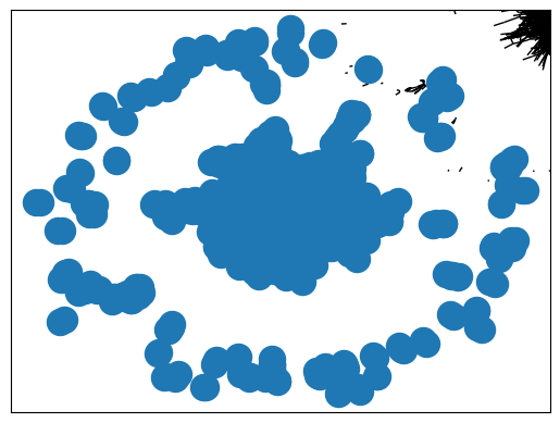

PyG has lots of interesting datasets, both from a ML point of view and from a visualization point of view. Below is generic approach to download the data and convert it to NetworkX and GML.

from torch_geometric.datasets import Amazon
import numpy as np
from scipy.sparse import coo_matrix
import networkx as nx
# the name can only be 'Computers' or 'Photo' in this case.
amazon = Amazon(root='~/Amazon', name="Computers");
edges = amazon.data["edge_index"];
row = edges[0].numpy();
column = edges[1].numpy();
data = np.repeat(1, edges.shape[1]);
adj = coo_matrix((data, (row, column)));
graph = nx.from_scipy_sparse_matrix(adj);
# nx.write_gexf(graph, "//graph.gml")

The COO format referred to is a way to store sparse matrices, see the SciPy documentation. As outline below, from here on you can use various tools to visualize the graph.

Neo4j

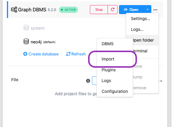
Download the two CSV files (nodes and edges) and put them in the import directory of the database (see screenshot). They can’t be in any other directory since Neo4j will not access files outside its scope.

Run the queries:

LOAD CSV WITH HEADERS FROM 'file:///nodes.csv' AS row
Create (n:Paper{id:row["nodeId"], subject:row["subject"], features:row["features"]});

LOAD CSV WITH HEADERS FROM 'file:///edges.csv' AS row
Match (u:Paper{id:row["sourceNodeId"]})
Match (v:Paper{id:row["targetNodeId"]})
Create (u)-[:Cites]->(v);

This creates something like 2708 nodes and 10556 edges. You can also directly download this Neo4j v5.2 database dump if you prefer.

Visualization

You can easily visualize the dataset with various tools. The easiest way is via the yEd Live by opening this GraphML file. There is also the desktop version of yEd.

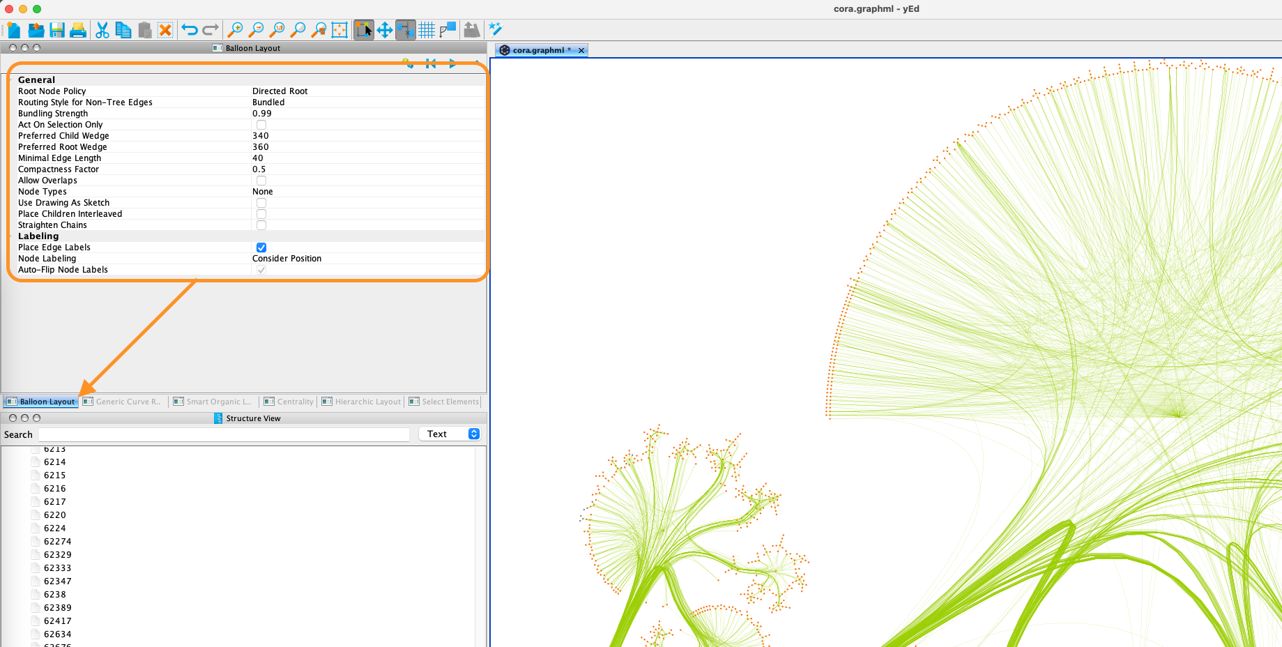
If you wish to reproduce the layout shown, use the balloon layout and use the settings shown below

The Gephi app is a popular (free) app to explore graphs but offers fewer graph layout algorithms. Use this Gephi file or import the aforementioned GraphML file.

Finally, there is Cytoscape and if you download the yFiles layout algorithms for Cytoscape you can create beautiful visualizations with little effort.