# not a must for this simple example but in general good to have GPUs when doing graph ML
!nvidia-smi -L


# Add this in a Google Colab cell to install the correct version of Pytorch Geometric.
# Torch Scatter can in particular be a frustrating experience
import torch

def format_pytorch_version(version):
  return version.split('+')[0]

TORCH_version = torch.__version__
TORCH = format_pytorch_version(TORCH_version)

def format_cuda_version(version):
  return 'cu' + version.replace('.', '')

CUDA_version = torch.version.cuda
CUDA = format_cuda_version(CUDA_version)

!pip install torch-scatter -f https://data.pyg.org/whl/torch-{TORCH}+{CUDA}.html
!pip install torch-sparse -f https://data.pyg.org/whl/torch-{TORCH}+{CUDA}.html
!pip install torch-cluster -f https://data.pyg.org/whl/torch-{TORCH}+{CUDA}.html
!pip install torch-spline-conv -f https://data.pyg.org/whl/torch-{TORCH}+{CUDA}.html
!pip install torch-geometricBarbell Embedding with PyG
PyG
The Barbell graph is an interesting graph to look at with respect to node embeddings because it has two distinctive blobs which should get emnedded in latent space in two clusters. Simply said, the graph visual and its embedding should be very similar.
Barbell Embedding with PyG
The Barbell graph is an interesting graph to look at with respect to node embeddings because it has two distinctive blobs which should get emnedded in latent space in two clusters. Simply said, the graph visual and its embedding should be very similar. This is only true if you don’t have a payload on the nodes and the embedding is purely based on the topology. The notebook explores this idea and gives at the same time an example of how to approach node embeddings with Pytorch Geometric.
![]()
Let’s render the Barbell graph so you have an idea how it looks like
import matplotlib.pyplot as plt
import networkx as nx
import numpy as np
import pandas as pd
import seaborn as sns
import torch
from sklearn.decomposition import PCA
from tqdm import tqdm

pd.set_option('display.max_columns', None)
pd.set_option('display.float_format', lambda x: '%.4f' % x)
graph = nx.barbell_graph(15, 3)
nx.draw_networkx(graph, label=True)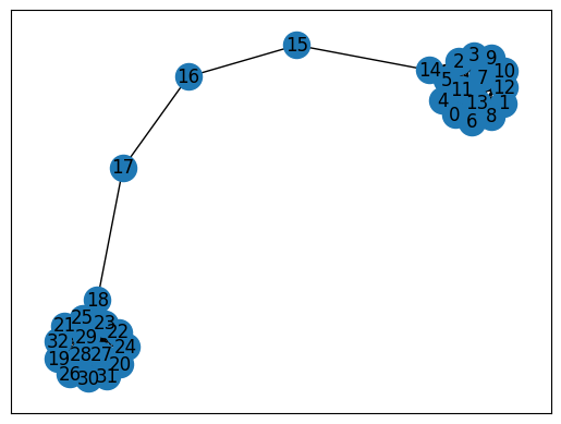
The embedding should resemble this layout with the intermediate nodes somewhere hanging between two clusters.
N = graph.number_of_nodes()
embedding_dim = 30
EPS = 1e-15
embedding = torch.nn.Embedding(N, embedding_dim)
optimizer = torch.optim.Adam(list(embedding.parameters()), lr=0.01)
The embedding parameters should be optimized so that the vectors (embedding the nodes) should be close if there is an edge between them. Note that there is no linear layers or weight matrix or anything else, it’s purely adjusting the embedding vectors.
def train():
    embedding.train()
    loss = 0
    for (u, v) in graph.edges:
        z_u = embedding.weight[u]
        z_v = embedding.weight[v]

        out = (z_u * z_v).sum(dim=-1).view(-1)
        pos_loss = -torch.log(torch.sigmoid(out) + EPS).mean()
        loss += pos_loss
    loss.backward()
    optimizer.step()
    return loss.item()

for e in range(1, 201):
    loss = train()
    if e % 10 == 0:
        print(f"epoch: {e}, loss: {loss}")
epoch: 10, loss: 350.039306640625
epoch: 20, loss: 192.37416076660156
epoch: 30, loss: 81.0612564086914
epoch: 40, loss: 20.464614868164062
epoch: 50, loss: 2.725670576095581
epoch: 60, loss: 0.14878813922405243
epoch: 70, loss: 0.011140757240355015
epoch: 80, loss: 0.00128898024559021
epoch: 90, loss: 0.00021363147243391722
epoch: 100, loss: 6.902414315845817e-05
epoch: 110, loss: 3.3379146771039814e-05
epoch: 120, loss: 1.8358399756834842e-05
epoch: 130, loss: 1.0848104466276709e-05
epoch: 140, loss: 6.7949526965094265e-06
epoch: 150, loss: 4.410753263073275e-06
epoch: 160, loss: 3.099446303167497e-06
epoch: 170, loss: 2.2649790025752736e-06
epoch: 180, loss: 1.7881409348774469e-06
epoch: 190, loss: 1.4305124977909145e-06
epoch: 200, loss: 1.1920935776288388e-06It takes effectively less than a hundred epochs to adjust things because the amount of data is so small. If we now render the 30-dimensional vectors with PCA we get:
@torch.no_grad()
def plot_embedding(embedding, title="Barbell embedding"):
    plt.figure()
    pca = PCA(n_components=2)
    z = pca.fit_transform(embedding.weight.numpy())
    sns.scatterplot(x=z[:, 0], y=z[:, 1], alpha=0.3, s=200)

    # show the label of each node on the figure
    for i, (x, y) in enumerate(z):
        plt.text(x, y, i)
    plt.title(title)

plot_embedding(embedding)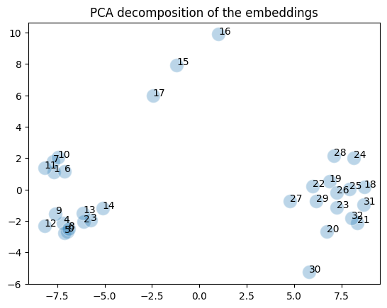
You can see that the two clusters neatly reflect the Barbell structure and the three intermediate nodes are hanging between the clusters. Note however that this is a projection of a 30 dimensional vector space that in reality this is not how the embedding looks like.
This is a simple embedding of the immediate neighborhood of a node. Every node attached a given one is pulling it in the embedding space. The interesting question is how to go beyond the 1-hop embedding, how to include a more of a node’s neighborhood? The challenge here is that if you go beyond the parents and children you get a set which can be very diverse: some nodes might have no 2-hop nodes, some might have a lot. Because machine learning can’t deal very well with varying (jagged) tensors, this poses a challenge. Either you have to pad tensors or you need to find a way to generate tensors of equal size. The padding leads to sparse vectors, which leads to the dimensionality curse. The generation of equal size tensor leads to a smart trick: the usage of random walks with predefind length. The random walk also solves the problem of dense graphs. If a node has a dense neighborhood or the neighborhoods are widely varying across a graph it would lead to lots of data harvesting. The random approach generates tensors of the same size and ensure that the collecting of data does not get out of hand. Of course, the random walk inevitable introduces randomness, the random walk potentially does not harvest the interesting adjacency. To remedy this the random walk is not purely random, the pseudo-random algorythm has two factors defining how close it stays to the starting point and how exotic it ventures downstream the graph.
The pseudo-random walk leads to n-hop embeddings and is more generic than the simple algorythm we used above. It also leads to the message-passing algorythms widely used in graph machine learning.
It’s interesting to note (on a more philosophical level) that randomness is a solution to a scalability problem. You trade certainty in for flexibility and universality.