About anyons

Quantum

What are anyons?

Keywords

Quantum Computing, Quantum Field Theory

The world around us consists of two families; bosons and fermions. The two families coexist in harmony but have a very different behavior, among other things their statistical behavior is different. On a quantum level this is noticeable when you try to swap two identical members; if you swap two bosons no blip but if you swap fermions you get a minus sign. The minus sign is, ultimately, the reason why our universe does not collapse (via the Pauli exclusion principle). So, one can effectively split the universe in a +1 family and a -1 family.

Things get weird when you travel from one dimension to another. It’s a scientific curiosity (pointed out by Hawking and Penrose) that one cannot have the same organic life in 2D as we have in 3D. Mammals fall apart in 2D.

A similar curiosity is that a 5D-being can escape any prison in 4D via a translation in time. The playing around with dimensions is a common technical trick in physics; dimensional regularization, dimensional analysis and so on. At the same time, certain models require higher dimensions, like superstrings and Kaluza-Klein theories. There are also interesting effects in nature when 3D things are constrained to lower dimensions and the effect of forcing electrons to move in a plane under intense magnetic field is one of them. The fractional quantum Hall effect creates via a collective effect quasi-particles (quarticles) which behave as if they do not belong to either fermions or bosons but something in between, hence the name any-ons. Rather than having +1 or -1 the particle get an arbitrary complex number \(e^{i\theta}\) when swapped.

The reason that one has anyons in 2D but not in 3D can be explained in various ways. The easiest conceptual explanation is that in three dimensions one can retract any loop to a point, even if there are point-like obstacle in space. Not so in a plane. Look at the picure below first in 3D and then in 2D; in the first case you can move the loop off the plane away from the point p but not in 2D.

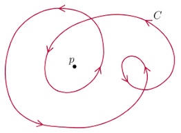
One says that the the homotopy group \(\pi_1\) is different. From a different perspective the issue can be casted in group theoretic language; the rotations in three or more dimensions has a double covering leading to the first homotopy group equal to \(\mathbb{Z}_2\). This directly translates to the existence of fermions and bosons. On the other hand, the first homotopy group of the rotations in two dimensions is equal to \(\mathbb{Z}\). When looking at permutations (i.e. swapping things) the permutation group in two dimensions becomes the first braid group while in three or more dimensions it has two irreducible one-dimensional representation (+1 and -1).

Identical things means that swapping them should have no effect. That’s only true in a classical world however, the Aharonov-Bohm effect shows that in quantum world it can induced a phase shift. If you look at the swapping in the image below you will understand that all of these changes have no effect in three or more dimensions because the paths can be retracted to a point while in 2D the complementary point is a topological obstruction.

The total wave function has a factor \(\Phi(\phi)\) which depends on the angle. In fact, from the point of view of the complementary particle the swapping is a loop of one around the other. The additivity of the factor \(\Phi(\phi)\) meands \(\Phi(\phi_1)\Phi(\phi_2) = \Phi(\phi_1 + \phi_2)\) and this only works with \(\Phi(\phi) = e^{i\eta\phi}\) with \(\eta\) an arbitrary real number. This matches with the Aharonov-Bohm factor of course. The arbitrary complex number (with modulus one) is what makes anyons special, you can have a swapping behavior that is neither bosonic nor fermionic but anything in between.

In order to describe an anyonic system it’s obvious that the usual Lagrangians (say, Maxwell or Klein-Gordon) will not do since they do not reproduce anyonic stats. At the same time there are not that many relativistic gauge-invariant Lagrangians out there. The Chern-Simons does the trick and we’ll show next how Abelian anyons make it happen.

Take the Abelian Chern-Simons dynamics bound to a matter current \(J\):

\[\mathcal{L}_{CS} = \frac{1}{2}\kappa\epsilon^{\alpha\beta\rho}A_\alpha\partial_\beta A_\rho - A_\mu J^\mu\]

This does not seem to be gauge invariant but if you assume the usual boundary conditions and \(\partial_\mu J^\mu = 0\) conservation it’s straighforward to see that \(A_\mu\mapsto A_\mu+\partial_\mu \Lambda\) induces

\[\frac{1}{2}\kappa\,\partial_\mu(\Lambda \epsilon^{\alpha\beta\rho}\partial_\beta A_\rho).\]

The Euler-Lagrange dynamics is

\[\frac{\delta \mathcal{L}_{CS}}{\delta A_\mu} = 0 = \frac{1}{2}\kappa\epsilon^{\alpha\beta\rho} F_{\beta\rho} - J^\alpha\]

or with the help of \(\epsilon^{\alpha\beta\sigma}\epsilon_{\alpha\mu\nu} = \delta^\beta_\mu\delta^\sigma_\nu - \delta^\sigma_\mu\delta^\beta_\nu\)

\[F_{\mu\nu} = \frac{\kappa}{2}\,\epsilon_{\mu\nu\rho}J^\rho.\]

If you set \(J = (\rho, \bar{J})\) and use the last equation in 2D you get

\[\begin{align}\rho & = \kappa B \\ J^i & = \kappa\epsilon^{ij} E_j\end{align}\]

with \(B\) the magnetic field and \(E\) the electric field. This result is a bit unusual since it says that the magnetic strength is proportional to the electric charge. This, however, is precisely what one needs to describe anynionic dynamics because if use electrons constrained to 2D you get a magnetic flux off the plane and through this a phase shift when looping around one another. So, let’s set

\[\rho(x,t) = e\sum_{a\in N} \delta(x - x_a(t))\]

describing \(N\) particles with worldline \(x_a\). The current density is correspondingly

\[\bar{j}(x,t) = e\sum_{a\in N} \dot{x}_a\,\delta(x - x_a(t))\]

and the (total) action of the system becomes

\[S = \frac{m}{2}\sum_a\int dt \,\bar{v}_a^2 +\frac{\kappa}{2}\int d^3x\,\epsilon^{\mu\nu\rho}\,A_\mu\partial_\nu A_\rho - \int d^3x\,A_\mu J^\mu.\]

As it stands we are still free to pick out any gauge we like, so let’s take \(A_0=0\) and \(\nabla \cdot A =0\). Recall that in two dimensions the Green function is

\[\Delta\left(\frac{1}{2\pi}\log|\bar{x}-\bar{y}|\right) = \delta^{(2)}(\bar{x}-\bar{y})\]

so the vector potential can be resolved to

\[A^i(\bar{x},t) = \frac{1}{2\pi\,\kappa}\int d^2y \,\epsilon^{ij}\frac{x^j-y^j}{|\bar{x}-\bar{y}|^2}\rho(\bar{y},t)\]

and with the density as above this reduces to

\[A^i(\bar{x},t) = \frac{e}{2\pi\kappa}\sum_a\epsilon^{ij}\frac{x^j-x^j_a(t)}{|\bar{x}-\bar{x}_a(t)|^2}.\]

From this the magnetic field can be computed and is indeed as seen earlier

\[B(\bar{x}_a) = \frac{e}{\kappa}\sum_{a\neq b}\delta(\bar{x}_a-\bar{x}_b)\]

and each anyon carries a flux \(\Phi = e/\kappa\). Finally, the phase shift from moving one anyon around another is given by the Wilson loop

\[\exp ie\oint A.dx = \exp\left(\frac{ie^2}{\kappa}\right).\]

This, in a nutshell, shows that Chern-Simons theory is the bridge between QFT and anyons.

The details of how anyons behave are however not necessary towards quantum computations. The situation is a bit similar to computing scattering amplitudes from Feynman diagrams rather than from first principles. In fact, how do anyons combine and interact? What happens when anyons split?

At this point we’ll assume that

there is a vacuum which we denote by 1
anyon and anti-anyon pairs can be created out of the vacuum (initialization)
interactions occurs in the shape of braid (a quantum algorithm)
the final state can be measured (result)

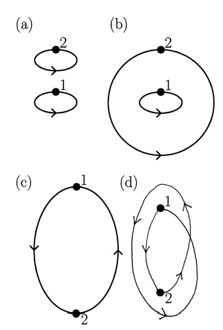
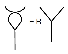
As a toy-example, imagine the anyon anti-anyon pair \(a, \bar{a}\). In standard QFT the following would be the same

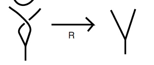
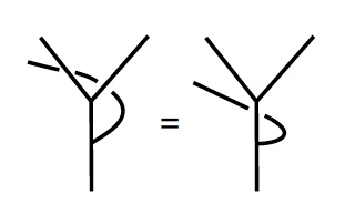
but in the case of anyons the twisting has an effect on the end-result. Also, in the following situation; can one map the results?

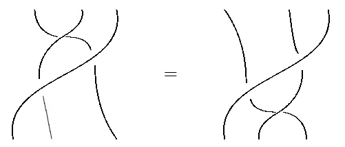
Recall that the n-dimensional Artin braid group \(B_n\) is defined as

\[\sigma_i\sigma_{i+1}\sigma_i= \sigma_{i+1}\sigma_i\sigma_{i+1} \\ \sigma_i\sigma_j =\sigma_j\sigma_i \;\text{if}\;|i-j|>1.\]

The first relation is called the Yang-Baxter relation and describes the equivalence of the diagram below

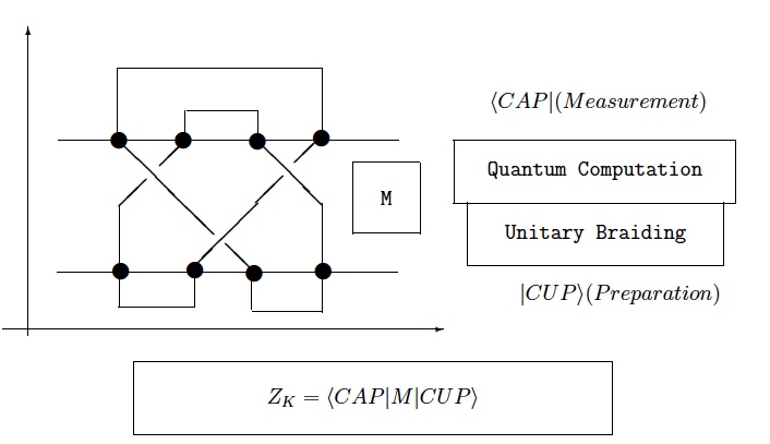
At this point at quantum algorithm can be seen as a representation of the braid group or as a representation of anyonic interactions. Let’s focus on the braid group first.

If we denote by \(R\) the swap of two particles the Yand-Baxter relation can be seen as an expression relating direct products:

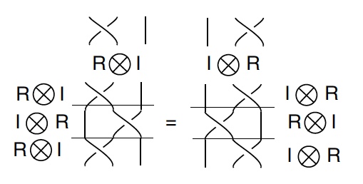
\[(R\otimes 1)(1\otimes R)(R\otimes 1) = (1\otimes R)(R\otimes 1)(1\otimes R).\]

The general solution of the Yang-Baxter relation is not easy but in the case of 4x4 matrices the generic solution can be one of the three matrices:

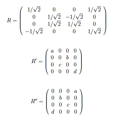
where \(a, b, c, d\) are unit complex numbers. If you take the standard basis \(\{|00\rangle\, |01\rangle\, |10\rangle\, |11\rangle\}\) you get for example

\[\begin{align} R|00\rangle &= \frac{1}{\sqrt{2}}|00\rangle - \frac{1}{\sqrt{2}}|11\rangle \\ R|01\rangle &= \frac{1}{\sqrt{2}}|01\rangle + \frac{1}{\sqrt{2}}|10\rangle \\ R|10\rangle &= -\frac{1}{\sqrt{2}}|01\rangle + \frac{1}{\sqrt{2}}|10\rangle \\ R|11\rangle &= \frac{1}{\sqrt{2}}|00\rangle + \frac{1}{\sqrt{2}}|11\rangle \\ \end{align}\]

which can be recognized as the Bell basis via an Hadamard transform. The general theorem this little computation suggests is the following theorem:

the \(R, R', R''\) are universal quantum gates.

The proof of this is not complex, see the wonderful articles by Louis Kauffman. The essence is this: there is an intimate connection between representations of the braid group and quantum algorithms (in the sense that such an algorithm is just a sequence of quantum gates). An even more fascinating result in this direction is the Brylinski theorem which says that any universal quantum gate has to be entangling and vice-versa. In other words, quantum algorithms are entangling qubits. Entanglement is the essence of quantum algorithms. Looking at famous examples like the Shor algorithm it’s quite obvious that the magic happens because of entanglement.

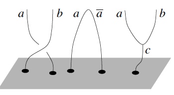
Returning to anyons and their interaction one can formalize general interactions by means of basic interactions as follows. The two pair creation processes are related by a linear mapping \(R\):

The intertwinning of three anyons as in the following diagrams are equivalent:

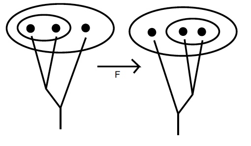
The double-splitting of anyons can also be mapped

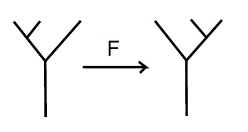
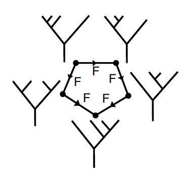
This is called a recoupling and the theory behind this is called recoupling theory. If you look at the recoupling figure and view it as a mirroring of the tree you will have no difficulty to recognize that if you use this on a tree with an extra branch you get the so-called pentagon identity:

Finally, if you combine the recoupling with the intertwinning identity you get a more involved hexagon identity:

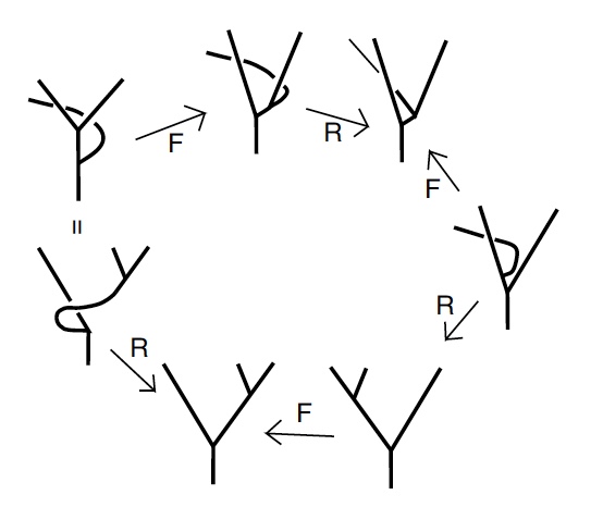
Just take a piece of paper and go through the steps one by one, it’s a lot of fun. Well, behind the fun there is a serious body of mathematics related to angular momenta, cobordism, category theory and spin networks.

Let’s look at a concrete example of recoupling, the so-called Fibonacci anyons. A Fibonacci anyon has only two types of interactions:

two anyons merge into the vacuum: \(a,a\mapsto 1\)
two anyons merge into a new one: \(a,a\mapsto a.\)

These rules are usually called fusion rules and one can summarize it in one line:

\[a\times a = 1 \times a\]

where you have to read it like you read the decomposition of direct group products \(3\otimes 3 \otimes 3 = 10 \oplus 8 \oplus 8 \oplus 1.\) How can one obtain an anyon from a fusion process using the Fibonacci rule?

0: if there is nothing it gives nothing
1: if there is one anyon you get one anyon
2: with two anyons there is only one way to get an anyon
3: in this case there are two ways to obtain an anyon (see figure)

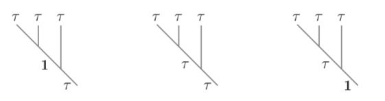
If you continue like this you notice that the next level depends on the previous one and the combinatorics reproduce the Fibonacci series, hence the name.

There is also another popular fusion model called the Ising anyonic model but the thinking is very much like the Fibonacci. See “A short introduction to Fibonacci anyon models” for more details.

In the next article we’ll go deeper on the relation between Chern-Simons and the Jones polynomial.