import networkx as nx
import pickle
with open('../data/EntityResolution.pkl', 'rb') as f:
    G = pickle.load(f)
print(G)
MultiDiGraph with 1237 nodes and 1819 edgesSee also this related note on how to use Jaccard in Neo4j via GDS.
Many companies use common sense when it comes to entity resolution:
These approaches work well in some cases but none of these techniques can access the topological information that every enterprise entity has. Some implicitly, sometimes explicit. That is, entities are never a data island, they always come with a cloud of information. This cloud of relations is a graph (network). Accurate entity resolution is, hence, a problem of not only matching the properties of an entity but also its context. The context augments the similarity and you should not omit it.
The reason companies don’t approach entity resolution from a graph point of view can have many origins:
and more. The transition from SQL to graphs can indeed be a project on its own and I have had customers deciding to avoid graphs knowing full well that it would increase accuracy, but increase cost in equal measures.
In this and subsequent notebooks we will try to explain various techniques to approach entity resolution. You can find vendor-specific articles about this but they (no surprise there) focus on their product and are usually focused on selling you a product rather than selling you a solution.
We’ll use a network originally from Neo4j (see this Github repo) and converted in NetworkX format here.
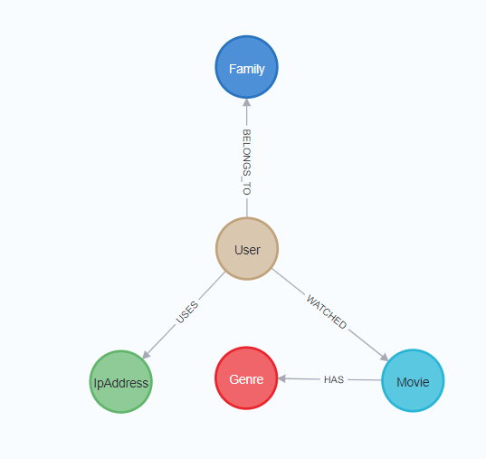
The schema is straightforward and the main objective is to consolidate users (label: User):
The data can be fetched from the pickle back into NetworkX like this:
import networkx as nx
import pickle
with open('../data/EntityResolution.pkl', 'rb') as f:
G = pickle.load(f)
print(G)MultiDiGraph with 1237 nodes and 1819 edgesThe data in the nodes consists of the usual suspects:
for id in G.nodes():
    print(G.nodes[id])
    break
{'labels': ['User'], 'properties': {'lastName': 'Burbidge', 'country': 'US', 'firstName': 'Dorette', 'gender': 'Male', 'phone': '834-424-8856', 'state': 'Ohio', 'userId': 1, 'email': 'dburbidge0@japanpost.jp'}}At mentioned above, common sense dictates to look at the properties to identify similarities. On a string level you have various options and Python has the built-in SequenceMatcher. Taking random pairs of User nodes and finding the similarity of the full names goes like this:
from difflib import SequenceMatcher
import random
# take the ids of the User labels
user_ids = [id for id in G.nodes() if "User" in G.nodes(data=True)[id]["labels"]]
pairs = [random.sample(user_ids , k=2) for _ in range(10)]
for pair in pairs:
    u = G.nodes(data=True)[pair[0]]["properties"]
    v = G.nodes(data=True)[pair[1]]["properties"]
    u_name = u["firstName"] + " " + u["lastName"]
    v_name = v["firstName"] + " " + v["lastName"]
    w = SequenceMatcher(None,u_name, v_name)
    print(u_name, v_name, w.ratio())
Nert Picopp Deni Jest 0.2
Konstanze Absolem Ronda Skilling 0.25806451612903225
Maxine Clousley Tarrah Caw 0.24
Port Prozescky Cacilie Nicklin 0.20689655172413793
Brana Cordeau Aurora Broadis 0.2962962962962963
Meryl Boncore Thedrick Dwine 0.37037037037037035
Riki Prujean Cece Brownstein 0.14814814814814814
Lynnelle Minkin Bar O'Hear 0.08
Carr Keemar Thedrick Dwine 0.24
Bobbe Wittering Maxine Francescone 0.24242424242424243This is not a practical solution because all possible pairs quickly grows with the amount of nodes. There is also the issue of missing data and how to impute, a classic data science problem.
The most basic topological similarity is based on the idea that the more friends you share, the more likely you know each other. The more two nodes share the same nodes in their 1-hop neighborhood, the more they are similar. This is expressed in the Jaccard similarity and is easy to compute. We are only interested in the similarity between User nodes, so we pass the index as the second paramter. Note that the given tuples have nothing to do with edges, we are only specifying which couples are interesting:
G = nx.Graph(G) # Jaccard will not work with multi-graphs
import itertools
user_combinations = list(itertools.combinations(user_ids, 2)) # around 125K combinations
jaccard_all_sim = nx.jaccard_coefficient(G, user_combinations)
jaccard_user_sim = [(u,v,w) for (u,v,w) in jaccard_all_sim if w>0.9]
for (u,v,w) in jaccard_user_sim:
    user_u = G.nodes[u]["properties"]
    user_v = G.nodes[v]["properties"]
    print(user_u["firstName"] + " " + user_u["lastName"], user_v["firstName"] + " " + user_v["lastName"], w)
Shirlene Borres Forrester Borres 1.0
Ondrea Garnsey Nadine Garnsey 1.0
Wanda W Wanda Wroath 1.0It’s important to stress here that the similarity is purely topological and does not depend on the properties of the nodes. That is, the method suggests that the nodes are similar because their neighborhood has some similarities.
In order to include the topology with the properties you need to step into graph machine learning and use node embeddings (node2vec).
Alternatively, you can use your heuristics together with the Jaccard coefficient to increase accuracy. Yet another road is to use classic machine learning and use the properties together with the topological similarity in your feature engineering.
For data scientist this topic is obvious but experience with customers shows that it’s much less clear to most people. So, here’s a note on features and how extra info can be used.
No matter the ML technique you use (SVM, XGBoost, neural networks…), you have a table with columns containing the characteristics of stuff and a special column (the target) that you wish to predict. If you wish to train an ML model which learns the similarity of nodes you collect the relevant properties that each node carries and you add it as a column. Since you have two nodes, you have these columns twice. The target column is a boolean saying whether they are or they are not similar. There are plenty of variations on this theme but let’s keep it simple.
The more rows you give to the algorithm, the more it will learn the characteristics of ‘the same’ two things (nodes).
Feature engineering is in this respect all about using meaningful features, combining them and converting them in a format suitable for ML. The important bit is also that you can add whatever you think can contribute to the process of detecting patterns. With (property) graphs you can add the payload of the nodes and edges AND the topological information. Provided you can encode the topology in a numerical format.
The way a node sits in a graph, the immediate neighborhood (1-hop) or a bit more (N-hops) can be encoded in a vector via a technique called node embeddings. In essence, a vector captures the neighborhood (topology) and this augments the features with information that a ML algorithm can use.
The creation of vectors from nodes (typically abbreviated as node2vec) is a topic we’ll explain elsewhere but there are various easy to use libraries which hide the complexity of assembling these vectors. The best known one is Node2Vec (pip install node2vec) or a faster version fastnode2vec (pip install fastnode2vec) with linear memory usage.
To create an embedding you need to convert the graph to another type of graph (since fastnode2vec inherits from the Gensim framework), define the parameters and train things:
from fastnode2vec import Graph, Node2Vec
graph = Graph(list(G.edges()), directed=True, weighted=False)
n2v = Node2Vec(graph, dim=10, walk_length=2, window=10, p=2.0, q=0.5, workers=2)
n2v.train(epochs=100)
This happens in less than a second and you can fetch node vectors like so:
print(n2v.wv[user_ids[0]])[ 0.00309572 -0.07105517 0.03536741 -0.00647308 0.0246973 0.01980644
-0.10460257 0.01136639 0.05422755 -0.06904547]With this in place we can start to use the vectors and the easiest thing is to use cosine similarity. Since the created vectors are Numpy arrays this is straightforward:
import numpy as np

def cosim(id_1, id_2):
    v1 = n2v.wv[id_1]
    v2 = n2v.wv[id_2]
    dot_product = np.dot(v1, v2)
    norm_a = np.linalg.norm(v1)
    norm_b = np.linalg.norm(v2)
    return dot_product / (norm_a * norm_b)

print(f"Cosine Similarity: {cosim(user_ids[1], user_ids[2]):.4f}")
Cosine Similarity: 0.4215Cosine similarity is really a mathematical translation for how close two vectors are to one another. The closer the value is to 1.0 the more they are close. The vector embedding ensures that vectors are close if the their topologies are similar and so, if we find high cosine values it means the two nodes have similar neighborhoods.
Once again, we look at the user nodes:
user_combinations = list(itertools.combinations(user_ids, 2))
cosim_users = [(u,v, cosim(u,v)) for (u,v) in user_combinations if cosim(u,v) > 0.9 ]
print(len(cosim_users))21In decreasing similarity:
sorted_cosim_users = sorted(cosim_users, key=lambda x: x[2], reverse=True)

# Iterate through the sorted list
for (u, v, w) in sorted_cosim_users[:10]:
    user_u = G.nodes[u]["properties"]
    user_v = G.nodes[v]["properties"]
    print(user_u["firstName"] + " " + user_u["lastName"], user_v["firstName"] + " " + user_v["lastName"], w)
Wandis Blewett Kristian Twaits 0.96341246
Riki Prujean Huey Ferneyhough 0.95864064
Eal Grombridge Konstanze Absolem 0.9390747
Perceval Pilbury Berk Mauser 0.93898416
Morgan Mongenot Maurine Mesant 0.93397725
Tova Canton Christopher Cowmeadow 0.9336317
Robyn Haskett Christiana Goodey 0.9315399
Danyette Pinnigar Dalt Le Quesne 0.9289893
Gardiner Dudman Lexy Canton 0.92787033
Gerard Toy Loydie Regis 0.9258602You might wonder what is the advantage over the Jaccard method above. Especially since both methods only take the topology into account and none of the properties.
The embedding is more general:
walk_length parameter reveals that underneath the hood there is a random walk collecting information about a node’s neighborhood. By increading the walk’s size you increase the size of the topology taken into account. The Jaccard method is 1-hop only. The additional paramters (p,q above) also are related to the random walk (how adventurous or exotic the walk is).One could say that Jaccard is the simplistic measure and Node2Vec fits in the AI (neural network) space. Whether one is better than the other depends on your tech stack, team, amount of data and so on.