from sympy import *
import math
from sympy.physics.quantum.circuitplot import CircuitPlot,labeller,Mz,CreateOneQubitGate
from sympy.physics.quantum.gate import *
from sympy.physics.quantum.qasm import Qasm
from sympy.physics.quantum.qapply import qapply
from sympy.physics.quantum.qubit import Qubit
from sympy.physics.quantum.state import *
from sympy.physics.quantum.dagger import Dagger
import matplotlib.pyplot as plt
%matplotlib inline
init_printing()


epr = qapply(Qubit('00') + Qubit('11'))/sqrt(2)

q0 = qapply(1*epr)
q1 = qapply(X(0)*epr)
q2 = qapply(Z(0)*epr)
q3 = qapply(Y(0)*epr)

T = H(1)*CNOT(1,0)
p0 = qapply(T*q0)
p1 = qapply(T*q1)
p2 = qapply(T*q2)
p3 = qapply(T*q3)

print(p0,p1,p2,p3)Superdense coding
Quantum
Doubling information content via qubits.
Keywords
Quantum Computing, Quantum Field Theory
- I. Introduction
- II. Elements of quantum mechanics
- III. The electromagnetic field
- IV. The qubit
- V. Quantum gates
- VI. States and operators
- VII. Shor’s algorithm
- VIII. Quantum teleportation
- IX. The Deutsch algorithm
- X. The no-cloning theorem
- XI. About anyons
- XII. About SU(2)
- XIII. Teleportation topology
- XIV. The Simon algorithm
- XV. Superdense coding
- XVI. Chern-Simons theory
- XVII. The toric code
- REF. Some pointers
Superdense coding is another surprising technique which allows one to send two bits of information with only one qubit. Entanglement allows you to pack more information than a classic pair of bits.
Start with an EPR pair
\[|\,\psi\rangle = \frac{1}{2}(\left|\,00\,\right\rangle + \left|\,11\,\right\rangle )\]
and depending on which number (something between 0 and 3 with two cbits) you (Alice) wish to send over you apply one of the following transformations
\[\left|\,00\,\right\rangle \rightarrow \frac{ 1}{\sqrt{2}} \left({\left|00\right\rangle } + {\left|11\right\rangle }\right)\]
\[\left|\,01\,\right\rangle \rightarrow \frac{ X_{0}}{\sqrt{2}} \left({\left|00\right\rangle } + {\left|11\right\rangle }\right)\]
\[\left|\,10\,\right\rangle \rightarrow \frac{ Z_{0}}{\sqrt{2}} \left({\left|00\right\rangle } + {\left|11\right\rangle }\right)\]
\[\left|\,11\,\right\rangle \rightarrow \frac{ Y_{0}}{\sqrt{2}} \left({\left|00\right\rangle } + {\left|11\right\rangle }\right)\]
Next, send half of the entangled pair to your buddy (Bob) and he applies an \(H_1*CNOT\) transformation on the qubit.
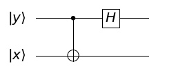
This results in \[\left|\,00\,\right\rangle \\ \left|\,01\,\right\rangle \\ \left|\,10\,\right\rangle \\ i\left|\,11\,\right\rangle \]
where the imaginary is just a phase factor and hence does not influence the measurment. The state can be measured in the Hadamard base and, hence, gives the two classical bits.
General dense coding schemes can be formulated in the language used to describe quantum channels. Alice and Bob share a maximally entangled state \(\omega\). Let the subsystems initially possessed by Alice and Bob be labeled 1 and 2, respectively. To transmit the message \(x\), Alice applies an appropriate channel
\[\; \Phi_x\]
on subsystem 1. On the combined system, this is effected by
\[\omega \rightarrow (\Phi_x \otimes I)(\omega)\]
where ‘’I’’ denotes the identity map on subsystem 2. Alice then sends her subsystem to Bob, who performs a measurement on the combined system to recover the message. Let the ‘’effects’’ of Bob’s measurement be \(F_y\). The probability that Bob’s measuring apparatus registers the message ‘’y’’ is
\[\operatorname{Tr}\; (\Phi_x \otimes I)(\omega) \cdot F_y .\]
Therefore, to achieve the desired transmission, we require that
\[\operatorname{Tr}\; (\Phi_x \otimes I)(\omega) \cdot F_y = \delta_{xy}\]
where \(δ_{xy}\) is the Kronecker delta.
The code to simulate this is straightforward using SymPy