The toric code

How noise spoils it all.

Keywords

Quantum Computing, Quantum Field Theory

• I. Introduction
• II. Elements of quantum mechanics
• III. The electromagnetic field
• IV. The qubit
• V. Quantum gates
• VI. States and operators
• VII. Shor’s algorithm
• VIII. Quantum teleportation
• IX. The Deutsch algorithm
• X. The no-cloning theorem
• XI. About anyons
• XII. About SU(2)
• XIII. Teleportation topology
• XIV. The Simon algorithm
• XV. Superdense coding
• XVI. Chern-Simons theory
• XVII. The toric code
• REF. Some pointers

Storing or manipulating information with a real physical system is naturally subject to errors. To obtain a reliable outcome from a quantum computation one needs to be certain that the processed information remains resilient to errors at all times. Overcoming errors means to detect and correct them continuously. The error detection process is based on an active monitoring of the system and the possibility of identifying errors without destroying the encoded information. Error correction employs the error detection outcome and performs the appropriate steps to correct it, thus reconstructing the original information.

Because cloning does not work on a quantum level (remember the quantum no-cloning theorym) one cannot use redundancy as one would on a classical level. So, the principle of quantum error correction is to encode information in a sophisticated way that gives the ability to monitor and correct errors. More concretely, the encoding is performed nonlocally such that errors, assumed to act in a local way, can be identified and then corrected without accessing the non-local information. Much like other quantum algorithms one makes use of entanglement but the toric code below goes a step further and uses topological information. The toric code is in fact

• a fun toy model demonstrating how anyons show up as excitations of a concrete (loop) ground state
• how the fusion rules we explained earlier correspond to a physical process
• how loops and Wilson lines (integrals) can encode information
• how quantum fluctuations can be corrected as a sympton detected by Hamiltonian dynamics.

The toric code is a particular example of what is known as quantum double models. Quantum double models are particular lattice realisations of topological systems. They are based on a finite group, G, that acts on spin states, defined on the links of the lattice. Based on these groups, stabiliser Hamiltonians can be defined consistently that have analytically tractable spectra. It can be shown that the ground states of these Hamiltonians behave like error correcting codes. Anyons are associated with properties of the spin states around each vertex or plaquette of the lattice. The fusion and braiding behaviour of the anyons depends on the property of the employed group, G. For example, an Abelian group leads to Abelian anyons and a non-Abelian group leads to to non-Abelian anyons. All the properties of the anyons emerge from the mathematical structure of the quantum double.

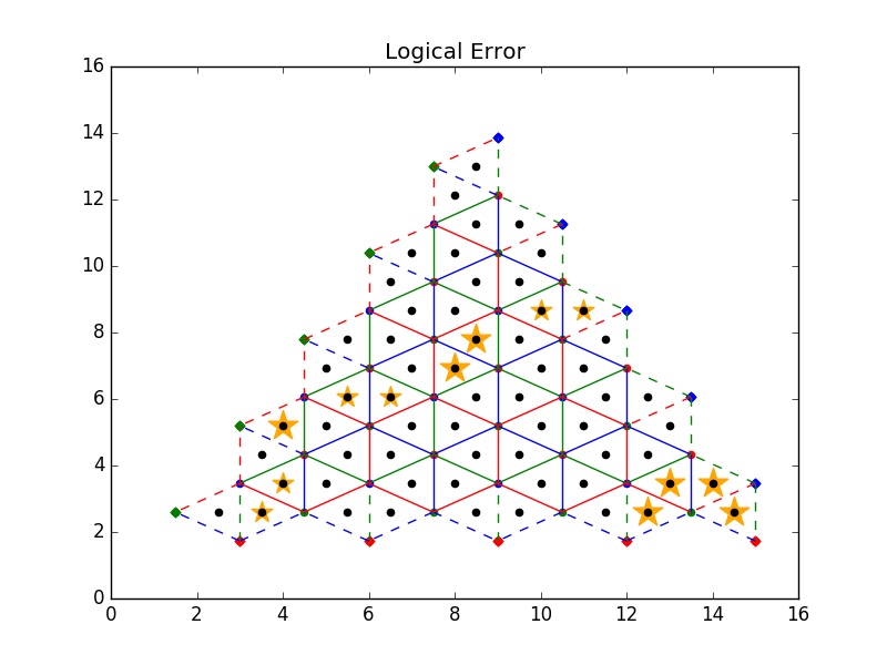
Before going into some details of the toric code I’d like to point out the cool QTop Python project allowing to simulate and visualize topological quantum codes. With just a few line one can instantiate a toric as well as a color code. A lot of fun.

Let’s consider a system of localized electrons that live on the edges of a square lattice. We’ll define the dynamics via the Hamiltonian

\[H = -A \sum_+ \prod_+\sigma_z - B \sum_\Box \prod_\Box\sigma_x\]

where the product in the first part is over the edges around a vertex and in the second part the edges of a plaquette.

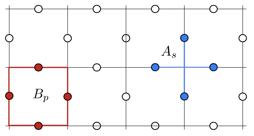
All the terms commute between themselves in this Hamilatonian. The only terms that you might suspect not to commute are a plaquette term and a vertex term that share some bonds. But you can convince yourself easily (by looking at the figure) that such terms always share an even number of spins. This means that the commutation picks up an even number of minus signs and so these terms commute as well.

Since the Hamiltonian is a sum of commuting terms, we can calculate the ground state \(\xi\) \[H\,|\xi\rangle = |\xi\rangle\]

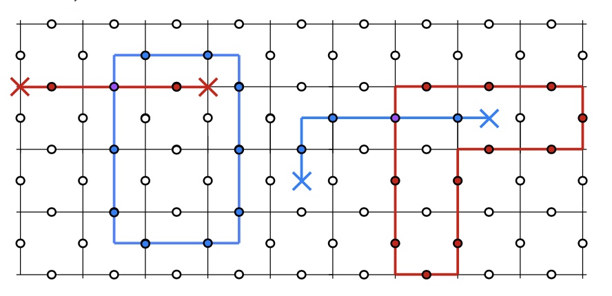
as the simultaneous ground state for all the terms. Let us first look at the vertex terms proportional to \(A\). If we draw a red line through bond connecting neighboring spins with \(\sigma_z=−1\) on our lattice (as shown below), then we find that each vertex in the ground state configuration has an even number of red lines coming in. Thus, we can think of the red lines forming loops that can never be open ended. This allows us to view the ground state of the toric code as a loop gas. You can also describe the ground state as one where both the vertex and plaquette operators give +1.

The loop gas can be divided in four sectors, corresponding to the homotopy

\[\pi_1(T_2) = \mathbb{Z}\times\mathbb{Z}\]

of the torus. If one uses the loops to store information it means that this four dimensional vector space can encode two qubits. One calls the ground state the stabilizer space of the code and the vectex/plaquette operators are called stabilizers.

One can get excitations of the vertex Hamiltonian by breaking loops. We can think of the end points of the loops as excitations, since the plaquette terms proportional to \(B\) make the plaquette terms fluctuate. These particles (that you see in the figure below) are called the electric defects, which we label ‘e’. As shown below, analogous defects in the \(\sigma_x\)-loops on the dual lattice are referred to as magnetic defects, which we will label ‘m’.

The Wilson operatos for these loops \(l_x\) and \(l_m\) are

\[W_e = \prod_{l_e}\sigma_z,\;W_m = \prod_{l_m}\sigma_x.\]

Hence \(W_e\) and \(_m\) are conserved ‘flux’ operators that measure the parity of the number of electric and magnetic defects inside the loops \(l_e, l_m\)respectively. Thus, the values \(W_{e,m}=-1\) can also be used to define what it means to have a localized ‘e’ or ‘m’ excitation respectively. These defects describe the localized excitations of the toric code. In fact in this model, this excitation on the ground states are localized to exactly one lattice site and may be viewed as point-like particles in a vacuum.

Since electrical vertex defects are produced in pairs and can be brought back together and annihilated in pairs we have

\[e\times x = 1\]

and similarly for the magnetic defects: \(m\times m = 1\). We might then wonder what happens if we bring together a vertex and a plaquette defect. They certainly do not annihilate, so we define another particle type, called \(f\), which is the fusion of the two

\[e\times m = f\]

and one has \(f\times f = 1\) because of associativity and commutativity

\[f\times f = (e\times m)\times (e\times m) = (e\times e)\times (m\times m) = 1.\]

Let us first consider the e particles. These are both created and moved around by applying \(\sigma_x\) operators. All of the \(\sigma_x\) operators commute with each other, so there should be no difference in what order we create, move, and annihilate the e particles. This necessarily implies that the e particles are bosons. There are several ”experiments” we can do to sow this fact. For example, we can create a pair of e’s move one around in a circle and reannihilate, then compare this to what happens if we put another e inside the loop before the experiment. We see that the presence of another e inside the loop does not alter the phase of moving the e around in a circle. The same logic applies to the magnetic excitations. In a word, the electric and magnetic particles are bosons.

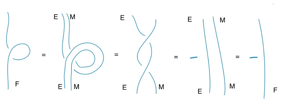
The proof that f on the other hand is a fermion is both beautifully simple and deep. It’s also a proof which combines a lot of what we tried to explain in previous articles: