Diffusion on graphs

The classic epidemic models on graphs.

import networkx as nx
import numpy as np
import random
import matplotlib.pyplot as plt

We will use Erdos-Renyi graphs and the Barabasi-Albert graphs as a basis for our diffusions:

N = 1500
k = 20
G1 = nx.erdos_renyi_graph(N, k/N)
G2 = nx.barabasi_albert_graph(N, k)
G3 = nx.gaussian_random_partition_graph(N,20,20,k/N,k/N)

SI model

The SI model is the simplest form of all disease models. Individuals are born into the simulation with no immunity (susceptible). Once infected and with no treatment, individuals stay infected and infectious throughout their life, and remain in contact with the susceptible population. This model matches the behavior of diseases like cytomegalovirus (CMV) or herpes.

In a continuous settings the model is defined via this set of coupled differential equations:

\[ \begin{align*} & \frac{d S}{dt} = -\frac{\beta S I}{N} \\ & \frac{d I}{dt} = \beta I (1 - \frac{I}{N}) \end{align*} \] with \(N = S + I\) the total population consisting of \(S\) susceptible individuals and \(I\) infected individuals. The factor \(\beta\) is the diffusion rate leading to a logistic growth of the infected population.

This simple diffusion model is really straightforward on a graph. Given a connection from an infected node to a susceptible one, a random value above a threshold (the diffusion parameter) defines whether or not the susceptible node gets affected. This loop runs untile the whole network is reached and infected. It’s also obvious that in this model the whole population gets infected eventually and this corresponds to the logistic curve as seen below.

def SI(G, initial_infected:int=1, beta:float=0.01, N:int=2000, T:int=1000):
    """
        Simulates the Susceptible-Infected (SI) model on a given graph.
        Parameters:
        G (networkx.Graph): The input graph where nodes represent individuals.
        initial_infected (int): The initial number of infected individuals.
        HM (float): The probability of infection transmission between connected nodes.
        N (int): The total number of individuals in the graph.
        T (int): The number of time steps to simulate.
        Returns:
        tuple: A tuple containing three numpy arrays:
            - susceptible (numpy.ndarray): The number of susceptible individuals at each time step.
            - infected (numpy.ndarray): The number of infected individuals at each time step.
            - infection_delta (numpy.ndarray): The number of new infections at each time step.

    """
    
    susceptible = np.zeros(T) # how many susceptible at time t
    infected = np.zeros(T) # how many infected at time t
    infection_delta = np.zeros(T) # increase in infection compared to previous time
    infected[0] = initial_infected
    susceptible[0] = N - initial_infected
    infection_delta[0] = infected[0]

    for u in G.nodes():
        G.nodes[u]["infected"] = 0
        G.nodes[u]["neighbors"] = [n for n in G.neighbors(u)]
    init = random.sample(G.nodes(), initial_infected)
    for u in init:
        G.nodes[u]["infected"] = 1

    for t in range(1,T):
        susceptible[t] = susceptible[t-1]
        infected[t] = infected[t-1]
        for u in G.nodes:            
            if G.nodes[u]["infected"] == 0:
                # nb_friend_infected = [G.nodes[n]["infected"] == 1 for n in G.nodes[u]["neighbors"]].count(True)
                for n in G.nodes[u]["neighbors"]:
                    if G.nodes[n]["infected"] == 1: 
                        # with HM infect
                        if np.random.rand() < beta:
                            G.nodes[u]["infected"] = 1
                            infected[t] += 1
                            susceptible[t] += -1
                            break
        infection_delta[t] = infected[t]-infected[t-1]
    return susceptible, infected, infection_delta

This is a simple implementation without using adjacency matrices or vectorizations. It ain’t the most performant one but it shows best what is going on.

Erdos Renyi

Let’s show explicitly what happens when using an Erdos-Renyi graph.

T = 100
N = 1500 
beta = 0.03
initial_infected = 2 

k = 20
G = nx.erdos_renyi_graph(N,k/N)
s_erdos, inf_erdos,infection_delta = SI(G,initial_infected,beta, N, T)
plt.plot((100/N)*s_erdos, color='b',marker='+', label="Susceptible p=0.04")
plt.plot((100/N)*inf_erdos, color='r',marker='o', label="Infected  p=0.04")
plt.xlabel("time")
plt.ylabel("Percentage of population infected")
plt.legend()
plt.show()

/var/folders/0p/dt9_dywj6rnc0wzps07dg31m0000gn/T/com.apple.shortcuts.mac-helper/ipykernel_47535/1712297490.py:28: DeprecationWarning: Sampling from a set deprecated
since Python 3.9 and will be removed in a subsequent version.
  init = random.sample(G.nodes(), initial_infected)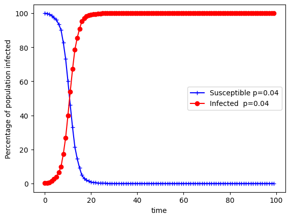

You can see that saturation happens extremely fast and this is due to the density of the network. If you reduce this you can see that some individuals don’t get infected because of the sparsity:

k = 3
T = 1000
G = nx.erdos_renyi_graph(N,k/N)
s_erdos, inf_erdos,infection_delta = SI(G,initial_infected,beta, N, T)
plt.plot((100/N)*s_erdos,"b",marker='+', label="Susceptible p=0.01")
plt.plot((100/N)*inf_erdos,"r",marker='o', label="Infected  p=0.01")

plt.xlabel("time")
plt.ylabel("% infected")
plt.legend()
plt.show()

/var/folders/0p/dt9_dywj6rnc0wzps07dg31m0000gn/T/com.apple.shortcuts.mac-helper/ipykernel_47535/1712297490.py:28: DeprecationWarning: Sampling from a set deprecated
since Python 3.9 and will be removed in a subsequent version.
  init = random.sample(G.nodes(), initial_infected)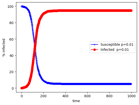

If you reduce \(k\) sufficiently there will be no infections at all. The problem will the model is that there is some randomness but given enoough time infection will always happen.

If we now look at infection delta’s you can see that there is an initial explosion of infections with a Poisson-like distribution:

k = 2 # the mean degree of the networks
# defining an erdos renyi network
G = nx.erdos_renyi_graph(N,k/N)
s_erdos, inf_erdos,infection_delta = SI(G,initial_infected,beta, N, T)
plt.plot(infection_delta,"r",marker='o', label="Infected  p=0.01")
plt.xlabel("time")
plt.ylabel("Number of new cases")
##

/var/folders/0p/dt9_dywj6rnc0wzps07dg31m0000gn/T/com.apple.shortcuts.mac-helper/ipykernel_47535/1712297490.py:28: DeprecationWarning: Sampling from a set deprecated
since Python 3.9 and will be removed in a subsequent version.
  init = random.sample(G.nodes(), initial_infected)

Text(0, 0.5, 'Number of new cases')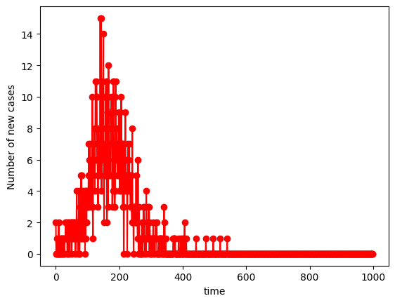

Barabasi-Albert

Let’s look at the Barabasi-Albert graph propagation:

k = 20
N = 500
initial_infected = 2

G1 = nx.erdos_renyi_graph(N,k/N)
G1_demi = nx.erdos_renyi_graph(N,k/N *0.5)
G2 = nx.barabasi_albert_graph(N, k)
G2_demi = nx.barabasi_albert_graph(N, int(k*0.5))

s_ER, inf_ER,nb_inf_t_ER = SI(G1,initial_infected,beta, N, T)
s_ER_demi, inf_ER_demi,nb_inf_t_ER_demi = SI(G1_demi,initial_infected,beta, N, T)

s_BA, inf_BA,nb_inf_t_BA = SI(G2,initial_infected,beta, N, T)
s_BA_demi, inf_BA_demi,nb_inf_t_BA_demi = SI(G2_demi,initial_infected,beta, N, T)
plt.figure(figsize=(15,10))
plt.plot(nb_inf_t_ER,"r", linewidth=2, label="Network:EA Infected  p=0.04")
plt.plot(nb_inf_t_ER_demi,"r--", linewidth=2, label="Network:EA Infected  p=0.02")


plt.plot(nb_inf_t_BA,"b", linewidth=2, label="Network:BA Infected  p=0.04")
plt.plot(nb_inf_t_BA_demi,"b--", linewidth=2, label="Network:BA Infected  p=0.02")
plt.xlabel("time")
plt.ylabel("Number of new cases")
plt.xlim(0,60)

plt.legend()
plt.show()

/var/folders/0p/dt9_dywj6rnc0wzps07dg31m0000gn/T/com.apple.shortcuts.mac-helper/ipykernel_47535/1712297490.py:28: DeprecationWarning: Sampling from a set deprecated
since Python 3.9 and will be removed in a subsequent version.
  init = random.sample(G.nodes(), initial_infected)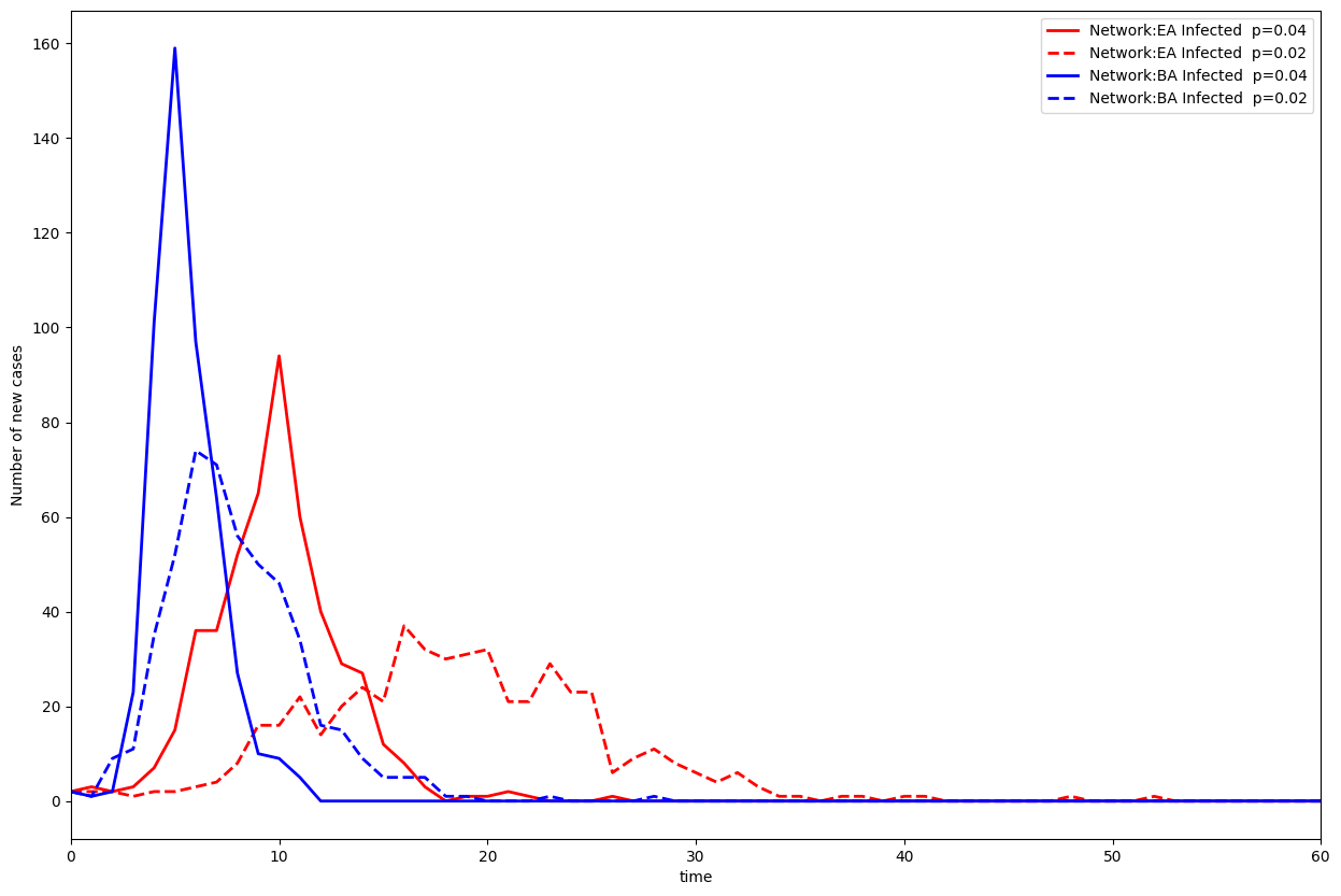

SIR model

The SI model is not satisfactory because everyone gets infected eventually and it does not take into account recovery, survival, removal (death) and so on. The SIR model improves the SI by adding a number of removed (and immune) or deceased individuals, denoted by \(R\):

\[ \begin{align*} & \frac{d S}{dt} = -\frac{\beta S I}{N}, \\ & \frac{d I}{dt} = \beta I S - \gamma I, \\ & \frac{d R}{dt} = \gamma I, \end{align*} \]

The \(\gamma\) coefficient corresponds to how fast an infection leads to deceased individuals.

def SIR(G, initial_infected, gamma, beta, N, T):
    
    susceptible = np.zeros(T)
    removed = np.zeros(T)
    infected = np.zeros(T)
    infected[0] = initial_infected
    susceptible[0] = N - initial_infected
    
    for u in G.nodes():
        G.nodes[u]["infected"] = 0
        G.nodes[u]["infectedDuration"] = 0
        G.nodes[u]["neighbors"] = [n for n in G.neighbors(u)]

    init = random.sample(G.nodes(), initial_infected)
    for u in init:
        G.nodes[u]["infected"] = 1
        G.nodes[u]["infectedDuration"] = 1
    # running simulation
    for t in range(1,T):
        susceptible[t] = susceptible[t-1]
        infected[t] = infected[t-1]
        removed[t] = removed[t-1]
        # Check which persons have recovered
        for u in G.nodes:
            # if infected
            if G.nodes[u]["infected"] == 1:
                if G.nodes[u]["infectedDuration"] < gamma:
                    G.nodes[u]["infectedDuration"] += 1
                else:
                    G.nodes[u]["infected"] = 2 #"recovered"
                    removed[t] += 1
                    infected[t] += -1
        # check contagion    
        for u in G.nodes:
            #if susceptible
            if G.nodes[u]["infected"] == 0:
                nb_friend_infected = [G.nodes[n]["infected"] == 1 for n in G.nodes[u]["neighbors"]].count(True)
                #print(nb_friend_infected)
                for n in G.nodes[u]["neighbors"]:
                    if G.nodes[n]["infected"] == 1: # if friend is infected
                        # with HM infect
                        if np.random.rand() < beta:
                            G.nodes[u]["infected"] = 1
                            infected[t] += 1
                            susceptible[t] += -1
                            break
    
    return susceptible, infected,removed

Once again, this isn’t the most performant implementation but demonstrative.

If we apply the algorithm an Erdos-Renyin graph:

np.random.seed(0)
# time of simulation
T = 100
# number of agents
N = 5000
beta = 0.03
gamma = 5
initial_infected = 2
# mean degree of the networks
k = 20
# defining an erdos renyi network
G = nx.erdos_renyi_graph(N,k/N)

s_erdos, inf_erdos,r_erdos = SIR(G,initial_infected,gamma,beta, N, T)
#plt.plot((100/N)*s_erdos, color='b',marker='+', label="Susceptible k=20")
plt.plot((100/N)*inf_erdos, color='r',marker='+', label="Infected p=0.04")
plt.plot((100/N)*r_erdos, color='g',marker='+', label="Recovered p=0.04")

#
# mean degree of the networks
k = 10
# defining an erdos renyi network
G = nx.erdos_renyi_graph(N,k/N)

s_erdos, inf_erdos,r_erdos = SIR(G,initial_infected,gamma,beta, N, T)
#plt.plot((100/N)*s_erdos,color="b",marker='o',label="Susceptible k=10")
plt.plot((100/N)*inf_erdos,color="r",marker='o',label="Infected p=0.02")
plt.plot((100/N)*r_erdos,color='g',marker='o',label="Recovered p=0.02")

plt.xlabel("time")
plt.ylabel("Percentage of population infected")
plt.legend()
plt.show()

/var/folders/0p/dt9_dywj6rnc0wzps07dg31m0000gn/T/com.apple.shortcuts.mac-helper/ipykernel_47535/935179267.py:16: DeprecationWarning: Sampling from a set deprecated
since Python 3.9 and will be removed in a subsequent version.
  init = random.sample(G.nodes(), initial_infected)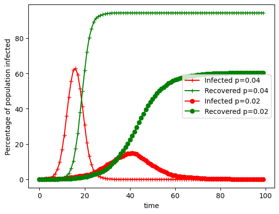

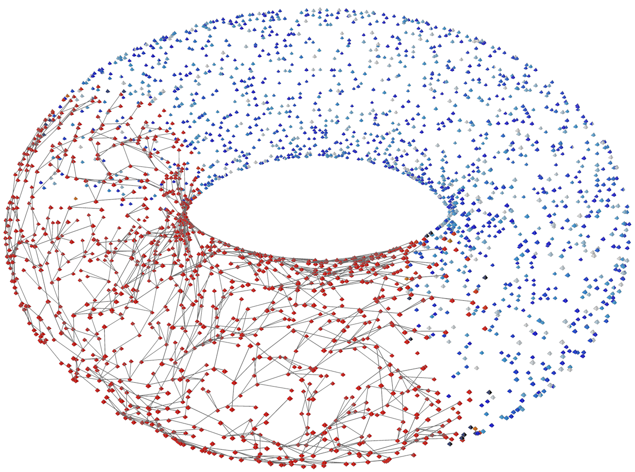
These epidemiology models are not limited to flat spaces and it’s interesting to apply it to other topologies, like a torus. In the adjacent image we used Python inside Cinema 4D to simulate infection: